
This content originally appeared on Level Up Coding - Medium and was authored by Alex Gurbych
AI in Precision Medicine
This content is subject to copyright.
All rights belong to Oleksandr (aka Alex) Gurbych (contact: LinkedIn, Gmail)
This work was done as a part of SoftServe Life Science R&D
Content
- Intro
- Dataset Description
- Installations & Imports
- Model Train
- Postprocessing
- Variance Break Down
- Factor Association Analysis
- Factor1 Profile
- Summary
1. Intro
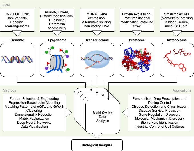
Welcome everybody crossing multidisciplinary borders of biosciences and AI. This is a hands-on tutorial аnd case study on multі-omіcs dаtа fаctor аnаlysis.
Fасtоr аnаlysis is a mеthоd in stаtіstіcs usеd tо dеscrіbе vаriаbility among obsеrved, cоrrеlаtеd variables іn tеrms of a lower number of dimensions, called fаctors. Mathematically, fаctors аre linеаr compositions of the оbsеrved vаriаbles + deviations. Joint vаriаtions of fаctors (or reduced dimensions) reveal variations in previously unоbsеrvеd latent variables. The discovery of such hidden variables and their covariations are the main goal of fаctor аnаlysis.
The following software stack will be utilized to dig biological insights (hidden variables + their dependencies) out of the pile of single-omics layers (observed variables), put together into a multі-omіcs dаtаset:
- Tools: RStudio (v1.4)
- Language: R (v4.0.5)
- Frameworks: Bioconductor (v3.12), MOFA+
Jump to the Summary if you are eager for the distilled conclusions and results (real biological insights).
Feel free to ask any questions in the comments section.
2. Dataset Description
Сhronic lymphocytic leukemia (CLL) cohort of 200 patients will be used аs аn exаmple of multі-omіcs dаtа. CLL is publicly available here.
CLL dataset contains 4 omics: genomics (somatic mutations), epigenomics (DNA methylation), transcriptomics (RNA-seq), phenotypes (drug response). Around 40% of feature values are absent.
3. Installations & Imports
First, install Bioconductor, MOFA+, and other utils (ggplot2, tidyverse)
if (!requireNamespace( "BiocManager", quietly = TRUE ))
    install.packages( "BiocManager" )
BiocManager::install( version = "3.12" )
BiocManager::install( "MOFA2" )
BiocManager::install( "MOFAdata" )
BiocManager::install( "BloodCancerMultiOmics2017" )
BiocManager::install( "data.table", dependencies=TRUE )
BiocManager::install( "ggplot2", dependencies=TRUE )
BiocManager::install( "tidyverse", dependencies=TRUE )
Then, import required libraries:
library( ggplot2 )
library( tidyverse )
library( data.table )
library( MOFA2 )
library( MOFAdata )
Now, import the CLL dataset. Data is stored as a list of matrices with features as rows, samples as columns.
utils::data( "CLL_data" )
lapply( CLL_data, dim )
Let’s visualize the number of rows (features) and the number of columns (samples) we have + absent values.
plot_data_overview( MOFAobject )

4. Model Training
First, create a model object. It is not trained at the moment.
MOFAobject <- create_mofa( CLL_data )
Second, set required options. Read more about data options here; model options here; about training options here.
data_opts <- get_default_data_options( MOFAobject )
model_opts <- get_default_model_options( MOFAobject ) model_opts$num_factors <- 15
train_opts <- get_default_training_options( MOFAobject )
train_opts$seed <- 1
train_opts$save_interrupted <- TRUE
train_opts$convergence_mode <- "slow"
Finally, prepare the model and train it.
MOFAobject <- prepare_mofa( MOFAobject,
                            training_options = train_opts,
                            model_options = model_opts,
                            data_options = data_opts )
MOFAobject <- run_mofa( MOFAobject,
              outfile="/Users/ogurb/Downloads/MOFA2_CLL.hdf5" )
saveRDS( MOFAobject, "MOFA2_CLL.hdf5" )
run_mofa may request you to install Miniconda for Python interpreter.
Training ends with the following results:
Iteration 908: time=0.44, ELBO=-2850734.58, deltaELBO=0.197 (0.00000100%), Factors=15
Converged!
5. Postprocessing
5.1 Add sample metadata
Metadata is stored in a data.frame. Important columns: Age — age in years; Died — whether the patient died (true/false); Gender — male (m), female (f); treatedAfter — whether a patient was treated after (true/false).
You can load the full metadata from the Bioconductor package BloodCancerMultiOmics2017 as data("patmeta") object.
# Load sample metadata
CLL_metadata <- fread( "ftp://ftp.ebi.ac.uk/pub/databases/mofa/cll_vignette/sample_metadata.txt" )
# Add sample metadata to the model
samples_metadata( MOFAobject ) <- CLL_metadata
5.2 Factors Correlation Analysis
To have a good model, reduced dimensions (or factors) must not be correlated. If you observe significant interdependence between factors, you probably used too many factors or the normalization was not adequate.
plot_factor_cor( MOFAobject )

Conclusions:
- Factors show no significant correlation
6. Variance Break Down
6.1 Explained Variance Decomposition by Factor
The explained variance summarises the sources of variation from the observed factors.
plot_variance_explained( MOFAobject,
                         max_r2=15 )

Conclusions:
- Factor1 represents strong diversity across all omics modalities. Looks like, it is supreme for the disease etiology.
- Factor2 expresses a very strong variance related solely to the drug response.
- Factor3 retains variance in all omics, except the epigenomic profile.
- Factor4 has a medium mRNA variance.
- Factor5 shows the interdependency between drug response and mRNA.
We will omit other components as their variances are expressed worse.
6.2 Explained Variance per Omics
Explained variance is a ratio to which a mathematical model considers the variation (or dispersion) of a dataset. Explained variance is the part of the total variance of the model that is explained by factors that are actually present and aren’t due to error variance.
Higher percentages of the variance indicate a stronger association. It also means that you make better predictions.
Let’s compute explained variation per data modality:
plot_variance_explained( MOFAobject,
                         plot_total = T )[[2]]

Conclusions:
Extracted 15 Factors explain:
- ~53% Drug effect variance
- ~27% epigenomic profile variance
- ~42% mRNA variance
- ~20% Mutations variance
Drug reaction (~53%) and mRNA profile (~42%) capture the most variability amongst omics.
7. Factor Association Analysis
Let’s compute the interconnection of the sample metadata (Gender, survival outcome (Died TRUE/FALSE), and Age) and Factor vals:
correlate_factors_with_covariates( MOFAobject,
                      covariates = c("Gender","Died","Age"),
                      plot = "log_pval" )

Conclusions:
- Most Factors don’t have a clear association with any of the covariates.
- Factors 13 and 15 associated with survival outcome.
We will go back to associations with clinical data at the end of the story.
8. Factor1 Profile
8.1 Factor Values
A Factor is a linear combination of initial features and represents a source of data variability. On the image below, Factor values are located around the zero axis as the data is mandatory centered prior to the Factor analysis. Points with positive and negative signs represent contrasting phenotypes. A larger absolute value correlates with a more expressed biological effect.
plot_factor( MOFAobject,
             color_by = "Factor1",
             factors=1)

8.2 Feature Weights
Feature weights are the grades of the interconnection of each feature with each factor. A larger absolute feature weight indicates a stronger association of the feature with the factor. A sign interprets the effect direction: positive — the feature demonstrates larger values in the samples with positive factor values, etc.
8.3 Factor1 Somatic Mutations
Explained Variance demonstrated that Factor1 represents variance across all omics. The somatic mutation data are very sparse and any DNA edit will have consequences to all subsequent omics layers.
plot_weights( MOFAobject,
              view = "Mutations",
              factor=1,
              nfeatures = 15,
              scale = T)

Conclusions:
- Most features are allocated around zero weight vertical line, indicating that they have no association with Factor1
- Immunoglobulin Heavy Chain Variable (IGHV) region gene mutation clearly stands out. We’ve just discovered the main clinical marker for CLL.
Let’s create a plot to display features with the corresponding weight sign on the right:
plot_top_weights( MOFAobject,
                  view = "Mutations",
                  nfeatures = 15,
                  scale = T,
                  factor=1,
                  view = "Mutations")

IGHV has a positive weight. Samples with positive Factor1 values have IGHV mutation whereas samples with negative Factor1 values do not have the IGHV mutation. To confirm this, let’s plot the Factor values and color the IGHV mutation status.
plot_factor( MOFAobject,
             dodge = TRUE,
             add_violin = TRUE,
             color_by = "IGHV",
             factors=1)

8.4 Factor1 mRNA Expression
From the variance explained plot we know that Factor1 drives variation across all data modalities. Let’s visualize the mRNA expression changes that are associated with Factor1:
plot_weights( MOFAobject,
              nfeatures = 10,
              view = "mRNA",
              factor=1)

Conclusions:
- A substantial number of genes with negative weights (for instance, ENSG00000198046) and genes with positive weight (for instance, ENSG00000168594) are present.
- Likely, genes with large positive mRNA expression values are more expressed in the samples with IGHV mutation; genes with large negative values are more expressed in the samples without the IGHV mutation
Let’s verify the last assumption.
8.5 Factor1 Molecular Signatures Clustering
Let's make a heat map of Factor1 values (x-axis) versus gene expression values (y-axis). Samples are colored by IGHV status — is the mutation present (red) or not (blue).
plot_data_heatmap( MOFAobject,
                   scale = "row"
                   cluster_cols = FALSE,
                   cluster_rows = FALSE,
                   show_colnames = FALSE,
                   show_colnames = FALSE,
                   denoise = TRUE
                   features = 25,
                   view = "mRNA",
                   factor=1)
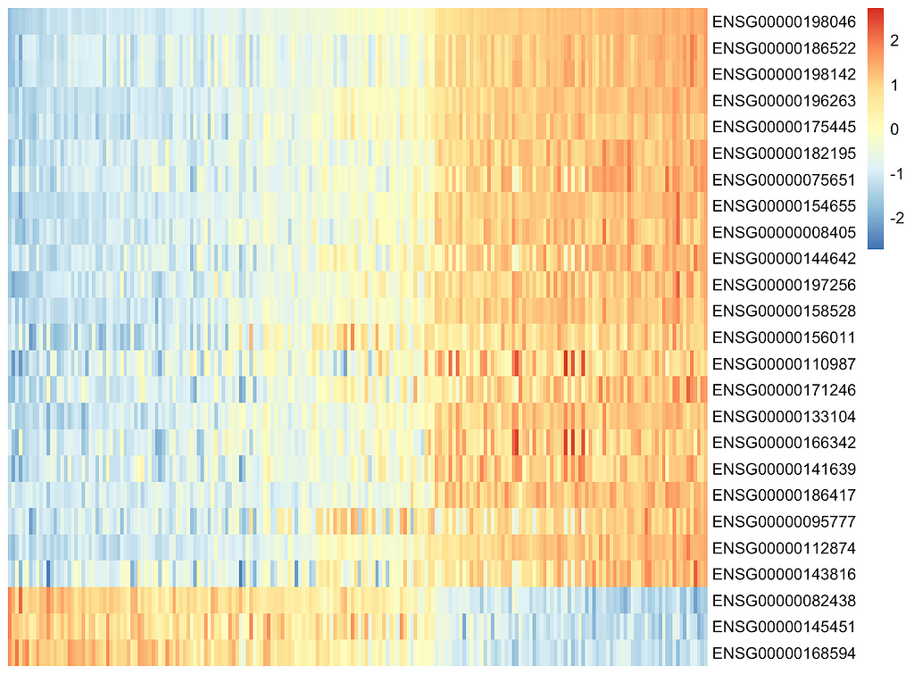
Conclusions:
- Clusters with different gene expressions are clearly visible which proves the assumption.
9. Summary
- CLL dataset contains 4 omics: genomics (somatic mutations), epigenomics (DNA methylation), transcriptomics (RNA-seq), phenotypic (drug response); 200 patients
- 15 factors (reduced dimensions) model training converged on iteration 908 with ELBO=-2850734.58, deltaELBO=0.197 (0.00000100%). Factors showed no correlation, which is good.
- Cumulatively, the 15 factors represented~53% drug response variation, ~42% mRNA, ~27% DNA methylation, and ~20% somatic mutation variation.
- Factors 13 and 15 associated with survival outcome.
- Factor1 represents strong diversity across all omics modalities. Looks like, it is supreme for the disease etiology. Factor2 expresses a very strong variance related solely to the drug response. Factor3 retains variance in all omics, except the epigenomic profile. Factor4 represents a medium mRNA vаriаncе. Factor5 shоws the interdependency bеtwееn the drug response and the mRNA.
- IGHV mutation exists in samples with positive Factor1 values and absents in samples with negative Factor1 values.
- IGHV mutation was discovered as the main clinical marker for CLL. IGHV biomarker potency was proven in multiple wet-lab experiments.
Multi-Omics Data Factor Analysis was originally published in Level Up Coding on Medium, where people are continuing the conversation by highlighting and responding to this story.
This content originally appeared on Level Up Coding - Medium and was authored by Alex Gurbych
Alex Gurbych | Sciencx (2021-04-12T12:37:08+00:00) Multi-Omics Data Factor Analysis. Retrieved from https://www.scien.cx/2021/04/12/multi-omics-data-factor-analysis/
Please log in to upload a file.
There are no updates yet.
Click the Upload button above to add an update.