
This content originally appeared on Level Up Coding - Medium and was authored by Anello
A detailed guide for Pre-Processing data in Machine Learning.

This first Machine Learning tutorial will cover the detailed and complete data pre-processing process in building Machine Learning models.
We’ll embrace pre-processing in data transformation, selection, dimensionality reduction, and sampling for machine learning throughout this tutorial. In another opportunity, we will apply this process with various algorithms to help you understand what it is and how to use Machine Learning with Python language.
Jupyter Notebook
See the Jupyter Notebook for the concepts we’ll cover on building machine learning models and my LinkedIn profile for other Data Science articles and tutorials.
First of all, we need to define the business problem. After all, we don’t create a machine learning model at random, although Machine Learning is fun in itself. We apply Machine Learning to solve a problem; it is a tool for solving business problems — from the issue or pain we want to address, we begin our work.
To say, dataset capture, variables transformation, the division of the training and test subsets, the learning and validation of the model depend on the definition of the business problem. Suppose we do not define the problem and do not specify it. In that case, we will simply be working randomly and creating a random model; after all the algorithms and techniques are chosen according to the dataset and the business problem.
Business problem: What’s your problem?
We will create a predictive model from the precise definition of the problem. We want to create a model that can predict whether or not a person can develop a disease — Diabetes.
For this, we will use historical patient data available in the Dataset: Pima Indians Diabetes Data Set that describes the medical records among Pima Indians patients. Each record is marked whether or not the patient developed Diabetes.
The set contains multivariate data, can be applied to time series, has categorical data, integer data, and 20 attributes.
Information about 9 main attributes:
- Number of times pregnant — X
- Plasma glucose concentration a 2 hours in an oral glucose — X
- Diastolic blood pressure (mm Hg) — X
- Triceps skin fold thickness (mm) — X
- 2-Hour serum insulin (mu U/ml) — X
- Body mass index (weight in kg/(height in m)²) — X
- Diabetes pedigree function — X
- Age (years) — X
- Class variable (0 or 1) — y
It is necessary a clear understanding of the variables. We need the predictor variables and the target variable so that we can work assertively with Machine Learning. And of course, from a lot of historical data to teach the algorithm, create a solid model, and make concrete predictions.
Once the business problem is defined, we need to search for the data to carry out our work. We will extract this data, load it into our analysis environment, and begin the exploration task. Let’s go…
Data source
This data can be in a CSV file, Excel spreadsheet, TXT file, in a relational or non-relational database table, in a Data Lake, Hadoop; that is, the data source can be the most varied! In general, the data engineer is responsible for extracting the data from the source and creating a pipeline. Therefore, a routine will be made to extract the data, store, process, and deliver the final result — usually, the data engineer is responsible for this process. The data scientist will receive this data in some format, upload it, and manipulate it.
Extract and load data
There are several considerations when uploading data to the Machine Learning process. For example: Do data have a header? If not, we’ll need to define a title for each column. Do the files have comments? What is the delimiter of the columns? Is data in single or double quotes? We must be aware of the details!
# Loading csv file using Pandas (method used use on this notebook)
from pandas import read_csv
file = 'pima-data.csv'
columns = ['preg', 'plas', 'pres', 'skin', 'test', 'mass', 'pedi', 'age', 'class']
data = read_csv(file, names = columns)
Instead of importing the entire pandas pack, we import only the read_csv from the Pandas library. This type of import consumes less computer memory.
Exploratory data analysis
After extracting and uploading the data, we perform exploratory analysis to understand the data we have available.
Descriptive statistics
First, let’s look at the first 20 rows of the set:
# Viewing the first 20 lines
data.head(20)

If the number of lines in the file is vast, the algorithm can take a long time to be trained, and If the number of records is too small, we may not have enough records to train the model. It is reasonable to have up to one million records for the machine to process without difficulty. Above that, the record numbers will demand computationally from the engine.
If we have many columns in the file, the algorithm can present performance problems due to the high dimensionality. In this case, we can apply the dimensionality reduction if necessary. The best solution will depend on each situation. Remember: train the model in a subset of the more extensive Dataset and then apply it to new data. That is, it is not necessary to use the entire Dataset. It is enough to use a representative subset to train the algorithm.
Check the dimensions of the Dataset
# Viewing dimensions
data.shape
(768, 9)
Check the Type of the Data
The type of data is essential. It may be necessary to convert strings, or columns with integers may represent categorical variables or ordinary values.
Identifying what each piece of data represents is the job of the data scientist. As much as we have numerical values, it may be that these columns represent categorical variables:
# Data type of each attribute
data.dtypes
preg       int64
plas       int64
pres       int64
skin       int64
test       int64
mass     float64
pedi     float64
age        int64
class      int64
dtype: object
Statistical Summary
# Statistical summary
data.describe()

In classification problems, it may be necessary to balance the classes. Unbalanced classes (more significant volumes of one of the class types) are common and need to be addressed during the pre-processing phase.
We can see below that there is an evident disproportion between classes 0 (non-occurrence of diabetes) and 1 (occurrence of diabetes).
We apply the class variable to the Pandas groupby function and measure its size:
# Class distribution
data.groupby('class').size()class
0    500
1    268
dtype: int64
We have 500 records with class 0 and 268 class 1 records, meaning we have more records of people who have not developed Diabetes than people who have developed. When the algorithm goes through these numbers, it will end up learning more about a person who does not have Diabetes than a person who has Diabetes — we need to have the same proportion for the two classes of the set.
One way to understand the relationship between data is through correlation. The Correlation is the relationship between 2 variables. The most common method for calculating correlation is the Pearson method, which assumes a normal distribution of data.
- A correlation of -1 shows a negative correlation, while
- A correlation of +1 shows a positive correlation.
- A correlation of 0 indicates that there is no relationship between the variables.
Some algorithms such as a linear regression and logistic regression can present performance problems with highly correlated (collinear) attributes.
How do I know if the algorithm requires modification? Consult the algorithm’s documentation to find out what the algorithm specifically needs
# Apply Pearson's correlation between all variables in the dataset data.corr(method = 'pearson')
We call the corr function and the Pearson method. We now have the correlation of each variable with all other variables.

What is relevant in the correlation’s return is to observe the value of the predictor variables concerning the target. Example: Age x Target — positive correlation, as you get older, the more likely you are to develop Diabetes.
Skew (or symmetry) refers to the distribution of data assumed to be normal or Gaussian (bell curve). Many Machine Learning algorithms assume that the data has a normal distribution. Knowing the symmetry of the data allows you to make a preparation and deliver what the algorithm expects to receive, thus increasing the predictive model’s accuracy.
Don’t expect the data to come ready to use. At some point, we need to modify the variables so that they have a format of a normal distribution — this does not mean changing the variable but changing the scale so that it can be in the normal distribution format.
# Checking each attribute's skew
data.skew()
preg     0.901674
plas     0.173754
pres    -1.843608
skin     0.109372
test     2.272251
mass    -0.428982
pedi     1.919911
age      1.129597
class    0.635017
dtype: float64
Here above, we have a symmetry index for each of the variables. We can understand how variables are distributed and decide if we will apply some normalization technique to put the variable in standard distribution format.
Matplotlib Visualization
We can bring to the exploratory analysis process the graphical tools offered by the Python language: matplotlib and seaborn.
First, we need to import matplotlib, specifically pyplot. The matplotlib inline is so that we can generate the graphics within the Jupyter Notebook window.
# It may be more interesting to generate the charts in a separate window as it is a set of smaller graphs
import matplotlib.pyplot as plt
%matplotlib inline
If we want to view the histogram more broadly in another window, we need to reset the Jupyter Notebook and remove the %matplotlib inline.
With the histogram, we can quickly assess the distribution of each attribute. Histograms group data into bins and provide a count of the number of observations in each bin.
We can quickly check the data’s symmetry with the histogram and whether it is in a normal distribution. It will help to identify outliers.
# Univariate Histogram
data.hist()
plt.show()

We can see that the attributes age, order, and test have an exponential distribution. We can see that the mass and press columns have a normal distribution.
We were able to obtain the same information by looking at the skew coefficients or by graphically observing the distribution of the variables.
Univariate Density plot
Density Plots are another way to visualize the distribution of data for each attribute. The plot is like a kind of abstract histogram with a smooth curve through the top of a histogram’s bins.
It may be easier to identify the distribution of the data using a density plot. The class seems to have two peaks because there are two classes — 0|1.
# Density Plot Univariate 'Density'
data.plot(kind = 'density',
          subplots = True,
          layout = (3,3),
          sharex = False)plt.show()

Box Plots
# Box and Whisker Plots
data.plot(kind = 'box',
          subplots = True,
          layout = (3,3),
          sharex = False,
          sharey = False)
plt.show()

With boxplots, we can also review the data distribution for each attribute. Boxplot helps to get an idea of the dispersion of the data and identifies outliers quickly: values that deviate a lot from the data’s average. If you leave the outlier in the dataset, it can affect the predictive model.
We can see that the dispersion of the data is quite different among the attributes. The age, skin, and test columns have symmetry very close to smaller data values.
# Box and Whisker Plots
data.plot(kind = 'box',
        subplots = True,
        layout = (3,3),
        sharex = False,
        sharey = False)
plt.show()
Let’s create a correlation matrix with the names of variables for easy visualization. The correlations object will receive all correlations in date through the corr() function.
Next, we call the NumPy library and plt.figure to create a figure. We add a subplot; then, we apply the matshow method to show the correlations between variables in a range from -1 to +1. After that, we use the color with fig.colorbar, create ticks with np.arange to set the square size at 9 (we have nine columns), and finalize, making adjustments to ticks and labels.
# Correlation matrix with variable names
correlations = data.corr()
import numpy as np
fig = plt.figure()
ax = fig.add_subplot(111)
cax = ax.matshow (correlations, vmin = -1, vmax = 1)
fig.colorbar(cax)
ticks = np.arange(0, 9, 1)
ax.set_xticks(ticks)
ax.set_yticks(ticks)
ax.set_xticklabels(columns)
ax.set_yticklabels(columns) plt.show() # Plot

This graph with matplotlib shows a correlation chart where intense yellow indicates a high correlation. In contrast, the darker color indicates a low correlation — an easier way to visualize the correlation between the data.
We can still create a generic correlation matrix, where the same procedure is done before, without applying labels. In this way, we can imply the creation of the correlation matrix.
# Simplified generic correlation matrix
correlations = data.corr()
fig = plt.figure()
ax = fig.add_subplot(111)
cax = ax.matshow(correlations, vmin = -1, vmax = 1)
fig.colorbar(cax)
plt.show()

Scatter Plot
To conclude, we can plot a scatter plot that will show the relationship between two variables as points in two dimensions, one axis being for each variable. Like the correlation matrix above, the scatterplot matrix is symmetric.
# Scatter Matrix
from pandas.plotting import scatter_matrix
scatter_matrix(data)
plt.show()

scatter_matrix()
Each square of the scatter matrix is a scatterplot showing the relationship of one variable to another.
Seaborn
Seaborn is a package for building statistical charts so that seaborn can widely use it during the exploratory phase of data with much more uncomplicated and leaner parameters.
import seaborn as sns
sns.pairplot(data)
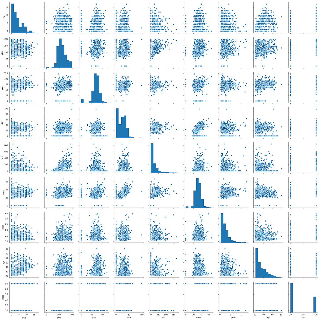
Seaborn pairplot is very similar to the matplot matrix scatterplot, but in a much easier way with a better finish. In the chart above, we were able to merge multiple charts into a single viewing area.
Seaborn boxplot
sns.boxplot(data = data, orient = "v")

See that the test variable is the one with the highest number of outliers. With a simple visualization, we have already been able to collect vital information.
Seaborn distplot
Finally, we have the distplot, calling only one variable from the dataset and using the fit parameter of the Stats module of the SciPy library.
from scipy import stats
sns.distplot(data.pedi, fit = stats.norm);

If you look right, we have three charts in a single plot. We have the histogram with an exponential distribution and some lines that help us put statistical summaries.
Therefore, this first exploratory step boils down to understanding the data. How the data is organized, the variables, the distributions of variables, the presence of outliers, the relationship of variables, etc.
Preparing the Data for Machine Learning
After performing the Exploratory Analysis to understand the data, we are ready to start the pre-processing step. This step embraces the transformation of the variables, selects the best ones for model creation, reduces the dimensionality for massive data sets, sampling, and other techniques depending on the data, business problem, or algorithm.
Many algorithms expect to receive data in a specific format. It is our job to prepare the data in a structure that is suitable for the algorithm we are using. The challenge is that each algorithm requires a different system, which may require other transformations in the data. But it is possible in some cases to obtain good results without pre-processing work.
Therefore, the important thing is not to decorate the process but rather to understand when it has to be done. As we work on different projects, the data may already arrive pre-processed.
Normalization — Method 1 (Scale)
Normalization, binarization, and standardization are techniques exclusively applied to quantitative variables. Normalization changes the scale of the data, and we have two techniques in scikit-learn; while standardization does not alter the distribution of data, it only places the distribution in a Gaussian format. That is, if the data is already in a normal distribution, we can only standardize it. And we still have binarization, which puts the data with the value 0 or 1 according to a rule that we specify.
It is one of the first tasks within the pre-processing. It is to put data on the same scale. Many Machine Learning algorithms will benefit from this and produce better results. This step is also called Normalization and means putting the data on a scale with a range between 0 and 1.
Normalization is valuable for optimization, being used in the core of the Machine Learning algorithms, such as gradient descent. It helps algorithms such as regression and neural networks and algorithms that use distance measurements, such as KNN. Scikit-learn has a function for this step, called MinMaxScaler ().
# Normalization (between 0 and 1)
from pandas import read_csv
from sklearn.preprocessing import MinMaxScaler
file = 'pima-data.csv'
columns = ['preg', 'plas', 'pres', 'skin', 'test', 'mass', 'pedi', 'age', 'class']
data = read_csv(file, names = columns)
array = data.values
X = array [:, 0: 8]
Y = array[:, 8]
scaler = MinMaxScaler(feature_range = (0, 1))
rescaledX = scaler.fit_transform (X)
print ("Original Data:", data.values)
print (" Standardized Data:", rescaledX [0: 5 ,:])
Here we transform the data to the same scale. We import the MinMaxScaler function for Normalization and read_csv function for reading the dataset. Next, we define the column names, pass the data values to an array, apply slicing in subsets, whereas the first eight columns are X predictors and the last column is the target variable y.
With the parameter feature_range of the MinMaxScaler function, we specify the scale between 0 and 1. After creating the scaler object, we use the fit process to apply the scaler to the X predictor data set — we do not need to normalize the output y variable in this case. That is, we use Normalization only to quantitative predictor variables.
Normalization — Method 2 (Scale)
This normalization method is a bit more advanced. It uses the normalizer function. In this case, we want to normalize the data, leaving it with a length of 1, creating a vector of length 1.
Therefore, here we used the method with Normalizer function instead of MinMaxScaler for normalizing variables:
# Normalization (length equal to 1)
from pandas import read_csv
from sklearn.preprocessing import Normalizer
file = 'data/pima-data.csv'
columns = ['preg', 'plas', 'pres', 'skin', 'test', 'mass', 'pedi', 'age', 'class']
data = read_csv(file, names = columns)
array = data.values
X = array[:,0:8]
Y = array[:,8]
print("Original data:", data.values)
print("Normalized data:", normalizedX[0:5,:])
Standardization (Standard Distribution)
Standardization is the technique for transforming attributes with Gaussian distribution and different means and standard deviations into a standard Gaussian distribution with the mean equal to 0 and standard deviation equal to 1.
The attributes of our dataset already have a normal distribution, only that this normal distribution presents different means and different standard deviation. The standardization will standardize the data with a mean 0 and standard deviation of 1.
Standardization helps algorithms that expect the data to have a Gaussian distribution, such as linear regression, logistic regression, and linear discriminant analysis. Works well when the data is already on the same scale. scikit-learn has a function for this step, called StandardScaler().
# Standardizing(0 for the mean, 1 for the standard deviation)
from pandas import read_csv
from sklearn.preprocessing import StandardScaler
scaler = StandardScaler().fit(X)
standardX = scaler.transform(X)
print("Original Data:", data.values)This data still represents the same information, but now the data distribution follows a standardized normal distribution.
Binarization (Transform data into 1 or 0)
As its name infers, it is a method for transforming data into binary values. We can set a limit value in our data, which we call a threshold, that will mark all values above the threshold will be marked as 1, and below the threshold will be marked as 0.
Binarization is useful when we have probabilities and want to turn the data into something with more meaning. scikit-learn has a function for this step, called Binarizer().
# Binarization
from pandas import read_csv
from sklearn.preprocessing import Binarizer
binarizer = Binarizer(threshold = 0.2).fit(X)
binaryX = binarizer.transform(X)
print("Original Data:", data.values)
print("Binarized Data:", binaryX[0:5,:])
Therefore, we have seen so far the chief standard techniques of data transfer: Normalization, Standardization, and Binarization.
Feature Selection
Once the variables are transformed, we can now select the best variables to build our model, which we call feature selection. In practice, we want to choose the best variables within the dataset to train a machine learning algorithm.
The attributes present in our dataset and that we use in the training data will significantly influence the predictive model’s accuracy and result. Unnecessary features will harm performance, while collinear characteristics can affect the rate of accuracy of the model. Eventually, we won’t know for ourselves what is irrelevant or not.
However, we have the opposite problem when we have two variables that represent the same information, which we call collinear attributes that can also impair the algorithm’s learning. Scikit-learn has functions that automate the work of extracting and selecting variables.
The feature selection step is to select the attributes (variables) that will be the best candidates for predictor variables. Feature Selection helps us reduce overfitting (when the algorithm learns extremely), increases model accuracy, and reduces training time. The idea is to create a generalizing model that takes Training Data and assumes any data set.
In our example, we have eight predictor variables and one target variable. Are the eight predictor variables relevant to our model? Keep in mind that the Machine Learning model must be generalizable; we can not create a model just for the training data. We need to create a model so that after it can receive new sets of data.
So we should try to get out of our front everything that might give us problems: irrelevant attributes or collinear attributes — it is not a simple task. In short, the selection of variables is made to select the essential variables for constructing the predictive model.
Univariate Statistical Tests for Feature Selection
Now we will see some techniques for picking variables. It is essential to consider that no method is perfect in creating each model; that is, we should look for the most appropriate technique of adapting the data to an algorithm to create the predictive model.
We may have a variable selection technique that presents a result, and after training the algorithm, we can notice that the outcome is not satisfactory. We go back to the beginning, try to find more adherent variables, compare the application of one technique with the other, and try it again. There is no perfection in this process.
Statistical tests can select attributes that have a strong relationship with the output variable (y — class) that we are trying to predict.
To teach the algorithm to predict this variable, we use all eight other predictor variables, but are they all relevant to predicting the target class variable? Therefore, we can use statistical tests that help us in the choices of these variables.
Scikit-learn provides the SelectKBest() function used with various statistical tests to select the optimal attributes (predictor variables — X). Let’s use the statistical chi-square test and select the four best features used as predictor variables.
In the Scikit-learn documentation, there is a list of all statistical tests offered by the SelectKBest() function.
# Extraction of Variables with Statistical Tests (Chi-Square Test)
from pandas import read_csv
from sklearn.feature_selection import SelectKBest
from sklearn.feature_selection import chi2
best_var = SelectKBest (score_func = chi2, k = 4)fit = best_var.fit(X, Y)features = fit.transform(X)
print('Original number of features:', X.shape[1])
print('Reduced number of features:', features.shape[1])
print('Features: nn', features)
First, we import the SelectKBest function and the chi2 statistical method of the feature_selection module. Then we load and split the data into X and y, and then we create the function to select the best variables.
Then, we call the SelectKbest function. We adjust the score_func parameter. The punctuation function will be chi2, and that this function will return the four most relevant attributes of the eight predictors we already have. Then we apply the fit to make the most pertinent relationship of X and y sets.
Once the fit is ready, we have the final fit object and transform it into X. That is, the fit object now represents which are the four best variables through the ratio of X and y. After this enhancement, the transform function will extract only the most relevant predictor X variables, and we will allocate them in the features object. Then the results are printed.
No model has been created so far, but with this method, we already know which variables are the most relevant.
Recursive Elimination of Attributes (RFE)
Within this technique, we will use Machine Learning to find the best predictor variables and then build the Machine Learning model, that is, to be able to extract in an automated way relevant information from the data set — the best predictor variables.
Recursive elimination is another technique for selecting attributes, which recursively removes features and constructs them with the remaining components. This technique uses the model’s accuracy to identify the characteristics that most contribute to predicting the target variable.
The example below uses the Recursive Attribute Elimination technique with a Logistic Regression algorithm to select the three best predictor variables. The RFE selected the variables “preg”, “mass” and “pedi”, which are marked as True in “Selected Attributes” and with value 1 in “Attribute Ranking.”
# Recursive Elimination of Variables
from pandas import read_csv
from sklearn.feature_selection import RFE
from sklearn.linear_model import LogisticRegression
file = 'data/pima-data.csv'
columns = ['preg', 'plas', 'pres', 'skin', 'test', 'mass', 'pedi', 'age', 'class']
data = read_csv(file, names = columns)
array = data.values
X = array[:,0:8]
Y = array[:,8]
model = LogisticRegression()
rfe = RFE(model, 3)
fit = rfe.fit(X, Y)
print("Predictor Variables:", data.columns[0:8])
print("Selected Variables: %s" % fit.support_)
print("Attribute Ranking: %s" % fit.ranking_)
print("Number of Best Attributes: %d" % fit.n_features_)
Here we import the RFE function of the feature_selecion module from the scikit-learn library to apply the variable selection technology and import the logistic regression algorithm from the linear_model.
Above, we load the data, make the slicing data set for the predictor and target variables, and instantiate the logistic regression model. Once the instance that owns the model name is created, we apply the RFE function; that is, we want to extract the 3 variables that most contribute to the accuracy of this predictive model for the rfe object. We generate the relationship of the X and y sets with the fit and print the result.
Extra Trees Classifier (ETC)
Here we will see another method of selecting variables using machine learning through an ensemble method — it is a category that encompasses a range of algorithms within a single algorithm. We feed this package of algorithms, the data is being distributed by these algorithms that make up the package and they are processing and making the predictions and at the end they vote to see which of those algorithms within the package has reached a more performative result. That is, several algorithms working in parallel and competing with each other to increase the accuracy of the result.
The algorithm in question is the Extra Trees Classifier, that is, a set of decision trees. ETC has the power to pick up multiple trees, place them inside a package, and in the end have an ensemble method to work with sorting — much like Random Forest.
Bagged Decision Trees, such as the RandomForest algorithm (these are called Ensemble Methods), can be used to estimate the importance of each attribute. This method returns a score for each feature. The higher the score, the greater the importance of the attribute.
# Importance of attribute with Extra Trees Classifier
from pandas import read_csv
from sklearn.ensemble import ExtraTreesClassifier
file = 'data/pima-data.csv'
columns = ['preg', 'plas', 'pres', 'skin', 'test', 'mass', 'pedi', 'age', 'class']
data = read_csv (file, names = columns)
array = data.values
X = array[:,0:8]
Y = array[:,8]
model = ExtraTreesClassifier()
model.fit(X, Y)
print(data.columns[0:8])
print(model.feature_importances_)
We created the ExtraTreesClassifier() model and related the X and y sets to the fit method, the training process. We take the ExtraTreesClassifier algorithm that already has its default parameters and present the data to it. Once this is done, we have the model created, trained, and listed the most relevant attributes.
These are the three main variable selection techniques: Univariate selection, recursive elimination, and ensemble method. Each of these methods can generate different variables since each method uses its parameters. It is up to the data scientist to choose what best suits the business problem and the available data — genuine engineering attributes.
Dimensionality Reduction
Within the data pre-processing step, we will now address dimensionality reduction after discussing the transformation and selection of variables. We will think about the recursive elimination of attributes. We had eight predictor variables, applied RFE recursive elimination, and the algorithm detected that three characteristics with greater relevance for constructing the model. With this in mind, we could discard the other five remaining attributes and use only the top 3 for model construction.
Although we are using the most relevant attributes, we discard attributes that may have some information. It may be irrelevant, but it’s still information; we could lose something no small. The method of selecting variables has its advantages, but it can also cause problems.
Therefore, we will see the reduction of dimensionality that instead of discarding the variables, we can encapsulate them in components through the PCA, one of the compression tools. That is, we take groups of variables and store them in components. This technique allows you to extract a small number of dimensional sets from a high-dimensional dataset. With fewer variables, the visualization also becomes much more meaningful. PCA is most useful when dealing with three or more dimensions.

In the graph on the left, we have the variables Gene1, Gene2, and Gene3. We can apply the PCA algorithm for unsupervised learning; that is, we do not know what the output is — The PCA will determine the patterns and group the data.
In the result on the right, the PCA creates the PC1 component and the PC2 component using multivariate statistical techniques. These components are groups of variables that have a very similar variance. Then we take these components and train the machine learning algorithm.
In general terms, PCA seeks to reduce the number of dimensions of a dataset by projecting the data into a new plan. Using this new projection, the original data, which can involve several variables, can be interpreted using fewer “dimensions.” In the reduced dataset, we can more clearly observe trends, patterns, and outliers. The PCA provides only more clarity to the pattern that is already there.
# Extraction Feature
from pandas import read_csv
from sklearn.preprocessing import MinMaxScaler
from sklearn.decomposition import PCA
file = 'data/pima-data.csv'
columns = ['preg', 'plas', 'pres', 'skin', 'test', 'mass', 'pedi', 'age', 'class']
data = read_csv (file, names = columns)
array = data.values
X = array[:,0:8]
Y = array[:,8]
scaler = MinMaxScaler(feature_range = (0, 1))
rescaledX = scaler.fit_transform(X)
pca = PCA(n_components = 4)
variancesfit = pca.fit (rescaledX)
print("Variance: %s" % fit.explained_variance_ratio_)
print(fit.components_)
Let’s call the MinMaxScaler function of the pre-processing module to normalize the data and the PCA algorithm of the decomposition module for dimensionality reduction. We load the data, separate the X and y sets, do normalization with MinMaxScaler establishing the range between 0 and 1, and apply the training to the X set.
Once normalized, we created the PCA by establishing four components we apply the PCA fit training to the normalized data. We have four components, the first component being the one with attributes of more significant variance, the second component of the second largest variance, and so on.
When we’re going to train the algorithm, we’re not going to introduce the algorithm to the dataset variables but the components. Thus, we were able to transmit all the information in the set so that the algorithm can achieve high accuracy. With highly dimensional datasets with more than 300 variables, we can reduce all of this to 150, 80, or 50 components to facilitate machine learning algorithm training. Therefore, PCA dimensionality reduction is a valuable pre-processing technique used according to the business problem.
Sampling
From now on, we’ll complete the pre-processing data step to move on to the following data science track. Sampling is an essential concept for dividing data into training data and test data. We must wonder whether we need to use the entire data set available to train the Machine Learning algorithm. Ideally, we will collect a sample from the dataset to train the algorithm and another piece to test the model’s performance.
We do this because we already have the historical data set. We collect in the past data from patients who have developed or not diabetes. We have several predictor variables and the output variable; that is, we already know the patients who developed the disease or not. We now want to teach the algorithm how to detect this for us in the future.
When training the algorithm with a data sample intended for training, we will test the algorithm with another piece of this data set; after all, we already know the result since we work with historical data. Therefore, we will compare the result of the model with what belongs to the test data and calculate the model’s error rate.
If we present the model data that we’ve never seen before, we don’t have a reference to measure model performance. Thus, we use the training data to train and use another sample to test the performance of the predictions and therefore evaluate the model according to the error rate generated.
# Evaluation using training and test data
from pandas import read_csv
from sklearn.model_selection import train_test_split
from sklearn.linear_model import LogisticRegression
file = 'data/pima-data.csv'
columns = ['preg', 'plas', 'pres', 'skin', 'test', 'mass', 'pedi', 'age', 'class']
data = read_csv(file, names = columns)
array = data.values
X = array[:,0:8]
Y = array[:,8]
test_size = 0.33
seed = 7
X_train, X_test, Y_train, Y_test = train_test_split(X, Y, test_size = test_size, random_state = seed)
model = LogisticRegression()
model.fit(X_train, Y_train)
result = model.score(X_test, Y_test)
print("Accuracy in Test Data: %.3f%%" % (result * 100.0))
To make this division of the sets, we will import the train_test_split function of the model_selection module and import the LogisticRegression model to create the Machine Learning model and then evaluate the model’s performance.
Once this is done, we load the data; we separate it with the slicing of the set that we did up to that instant, we define a test_size with the value 0.33 and specify a seed to reproduce an expected result.
Next, we call the train_test_split function of scikit-learn, we pass X and y as a parameter, we apply the test_size that was already defined just now, and the random_state equal to the seed set. This function train_test_split returns four values, so we need four variables.
Then we instantiate the model with the LogisticRegression algorithm and do the training with the training data generated by the train_test_split. Next, we call the score function to measure the model’s performance, calculate its score and return to accuracy. The accuracy of the model was 75%.
Accuracy is measured in the test data because the model has been trained with the training data, and we need to present a set of data that it has not yet seen but that we know to evaluate the performance. However, there is still an even more effective division technique, cross-validation.
Cross Validation — best performance results
Above, we saw how to randomly divide the data between training data and test data to assess the model’s performance. However, this procedure has a slight problem of staticity in the application of train_test_split; that is, it is a single static division.
With cross-validation, we can do this flexibly several times and repeatedly, i.e., do this same division over and over again to train and test our machine learning model — training and testing the algorithm continually.
This cross-validation usually increases model performance but requires more computational capacity. It would be like using train_test_split multiple times, requiring more computational resources depending on the dataset and improving model performance.
See the column of fold1, representing training x testing. Considering we have 100 lines in our data set, we would take 80% for training and 20% for testing.
In fold2, what was test set now becomes train set, and what was train is now a test, i.e., different selections are made randomly in our dataset. Several samples are collected, and for each fold, the training and testing procedure of the algorithm is applied — increasing performance.

After the entire standard process until the composition of the X and y sets, we will determine the number of folds in 10. In the example diagram above, the division was in 5 folds — there is no consensus regarding the value of k (number of folds); that is, it will depend on the problem and the set. If the number of folds does not result in an expected value, we only change until we reach a satisfactory result.
# Cross Validation
from pandas import read_csv
from sklearn.model_selection import KFold
from sklearn.model_selection import cross_val_score
from sklearn.linear_model import LogisticRegression
file = 'pima-data.csv'
columns = ['preg', 'plas', 'pres', 'skin', 'test', 'mass', 'pedi', 'age', 'class']
data = read_csv(file, names = columns)
array = data.values
X = array[:,0:8]
Y = array[:,8]
num_folds = 10
seed = 7
kfold = KFold(num_folds, True, random_state = seed)
model = LogisticRegression()
result = cross_val_score(model, X, Y, cv = kfold)
print("Final accuracy: %.3f%%" % (result.mean() * 100.0))The accuracy for this code was 77%. This procedure is slightly different from the static train_test_split that resulted in 75%; the only additional factor was applying KFold, which increased by 1% in terms of accuracy — this can be pretty significant if you consider a vast dataset.
Besides, in train_test_split, we train the algorithm with training data and test the score with test. In cross-validation, this is not necessary, it does this automatically by training and testing, and at the end, we apply an average of the result accuracy of cross_val_score.
Therefore, cross-validation has accuracy for each fold, and at the end, we take the average of all accuracies and assume as a result for the model’s performance. Any minimum gain inaccuracy can be significant. In contrast, we will have a longer time spent and computational processing.
Concluding
We have completed the data pre-processing step here. So far, we have worked on pre-processing tasks: transformation, selection, dimensionality reduction and sampling.
Much of our time has been spent in detail here. From now on, we can move on to the learning, evaluation, and prediction steps inherent in the Data Science process.
And there we have it. I hope you have found this helpful. Thank you for reading. ?
Data Pre-Processing in Machine Learning with ? Python + Notebook was originally published in Level Up Coding on Medium, where people are continuing the conversation by highlighting and responding to this story.
This content originally appeared on Level Up Coding - Medium and was authored by Anello
Anello | Sciencx (2021-04-20T17:06:21+00:00) Data Pre-Processing in Machine Learning with Python + Notebook. Retrieved from https://www.scien.cx/2021/04/20/data-pre-processing-in-machine-learning-with-python-notebook/
Please log in to upload a file.
There are no updates yet.
Click the Upload button above to add an update.