This content originally appeared on DEV Community and was authored by davidkohn88
Table of contents
- A primer on PostgreSQL aggregation (through pictures)
- Two-step aggregation in TimescaleDB hyperfunctions
- Why we use the two-step aggregate design pattern
- Two-step aggregation + continuous aggregates in TimescaleDB
- An example of how the two-step aggregate design impacts hyperfunctions’ code
- Summing it up
Get a primer on PostgreSQL aggregation, how PostgreSQL’s implementation inspired us as we built TimescaleDB hyperfunctions and its integrations with advanced TimescaleDB features – and what this means for developers.
At Timescale, our goal is to always focus on the developer experience, and we take great care to design our products and APIs to be developer-friendly. We believe that when our products are easy to use and accessible to a wide range of developers, we enable them to solve a breadth of different problems – and thus build solutions that solve big problems.
This focus on developer experience is why we made the decision early in the design of TimescaleDB to build on top of PostgreSQL. We believed then, as we do now, that building on the world’s fastest-growing database would have numerous benefits for our users.
Perhaps the biggest of these advantages is developer productivity: developers can use the tools and frameworks they know and love and bring all of their SQL skills and expertise.
Today, there are nearly three million active TimescaleDB databases running mission-critical time-series workloads across industries. Time-series data comes at you fast, sometimes generating millions of data points per second (read more about time-series data). Because of this volume and rate of information, time-series data is complex to query and analyze. We built TimescaleDB as a purpose-built relational database for time-series to reduce that complexity so that developers can focus on their applications.
So, we’re built with developer experience at our core, and we’ve continually released functionality to further this aim, including continuous aggregates, user-defined actions, informational views, and most recently, TimescaleDB hyperfunctions: a series of SQL functions within TimescaleDB that make it easier to manipulate and analyze time-series data in PostgreSQL with fewer lines of code.
To ensure we stay focused on developer experience as we plan new hyperfunctions features, we established a set of “design constraints” that guide our development decisions. Adhering to these guidelines ensures our APIs:
- Work within the SQL language (no new syntax, just functions and aggregates)
- Intuitive for new and experienced SQL users
- Useful for just a few rows of data and high-performance with billions of rows
- Play nicely with all TimescaleDB features, and ideally, makes them more useful to users
- Make fundamental things simple to make more advanced analyses possible
What does this look like in practice? In this post, I explain how these constraints led us to adopt two-step aggregation throughout TimescaleDB hyperfunctions, how two-step aggregates interact with other TimescaleDB features, and how PostgreSQL's internal aggregation API influenced our implementation.
When we talk about two-step aggregation, we mean the following calling convention:

Where we have an inner aggregate call:

We chose this design pattern over the more common - and seemingly simpler - one-step aggregation approach, in which a single function encapsulates the behavior of both the inner aggregate and outer accessor:

Read on for more on why the one-step aggregate approach quickly breaks down as you start doing more complex things (like composing functions into more advanced queries) and how, under the hood, almost all PostgreSQL aggregates do a version of two-step aggregation. You’ll learn how the PostgreSQL implementation inspired us as we built TimescaleDB hyperfunctions, continuous aggregates, and other advanced features – and what this means for developers.
If you’d like to get started with hyperfunctions right away, create your free trial account and start analyzing ?. (TimescaleDB hyperfunctions are pre-installed on every Timescale Forge instance, our hosted cloud-native relational time-series data platform).
A primer on PostgreSQL aggregation (through pictures)
When I first started learning about PostgreSQL 5 or 6 years ago (I was an electrochemist, and dealing with lots of battery data, as mentioned in my last post on time-weighted averages), I ran into some performance issues. I was trying to better understand what was going on inside the database in order to improve its performance – and that’s when I found Bruce Momjian’s talks on PostgreSQL Internals Through Pictures. Bruce is well known in the community for his insightful talks (and his penchant for bow ties), and his sessions were a revelation for me.
They’ve served as a foundation for my understanding of how PostgreSQL works ever since. He explained things so clearly, and I’ve always learned best when I can visualize what’s going on, so the “through pictures” part really helped - and stuck with - me.
So this next bit is my attempt to channel Bruce by explaining some PostgreSQL internals through pictures. Cinch up your bow ties and get ready for some learnin’.
 The author pays homage to Bruce Momjian (and looks rather pleased with himself because he’s managed to tie a bow tie on the first try).
PostgreSQL aggregates vs. functions
We have written about how we use custom functions and aggregates to extend SQL, but we haven’t exactly explained the difference between them.
The fundamental difference between an aggregate function and a “regular” function in SQL is that an aggregate produces a single result from a group of related rows, while a regular function produces a result for each row:
 In SQL, aggregates produce a result from multiple rows, while functions produce a result per row.
This is not to say that a function can’t have inputs from multiple columns; they just have to come from the same row.
Another way to think about it is that functions often act on rows, whereas aggregates act on columns. To illustrate this, let’s consider a theoretical table ’foo’ with two columns:
CREATE TABLE foo(
    bar DOUBLE PRECISION,
    baz DOUBLE PRECISION);
And just a few values, so we can easily see what’s going on:
INSERT INTO foo(bar, baz) VALUES (1.0, 2.0), (2.0, 4.0), (3.0, 6.0);
The function greatest() will produce the largest of the values in columns bar and baz for each row:
SELECT greatest(bar, baz) FROM foo;

 greatest
---------------
        2
        4
        6
Whereas the aggregate max() will produce the largest value from each column:
SELECT max(bar) as bar_max, max(baz) as baz_max FROM foo;

 bar_max | baz_max
---------|--------
       3 |       6
Using the above data, here’s a picture of what happens when we aggregate something:
 The `max()` aggregate gets the largest value from multiple rows.
The aggregate takes inputs from multiple rows and produces a single result. That’s the main difference between it and a function, but how does it do that? Let’s look at what it’s doing under the hood.
Aggregate internals: row-by-row
Under the hood, aggregates in PostgreSQL work row-by-row. But, then how does an aggregate know anything about the previous rows?
Well, an aggregate stores some state about the rows it has previously seen, and as the database sees new rows, it updates that internal state.
For the max() aggregate we’ve been discussing, the internal state is simply the largest value we’ve collected so far.
Let’s take this step-by-step.
When we start, our internal state is NULL because we haven’t seen any rows yet:
Then, we get our first row in:
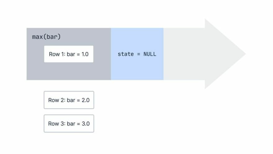
Since our state is NULL, we initialize it to the first value we see:
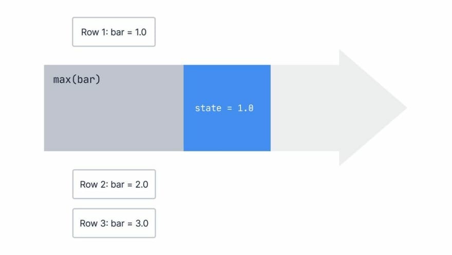
And we see that the value of bar (2.0) is greater than our current state (1.0), so we update the state:

Then, the next row comes into the aggregate:

We compare it to our current state, take the greatest value, and update our state:
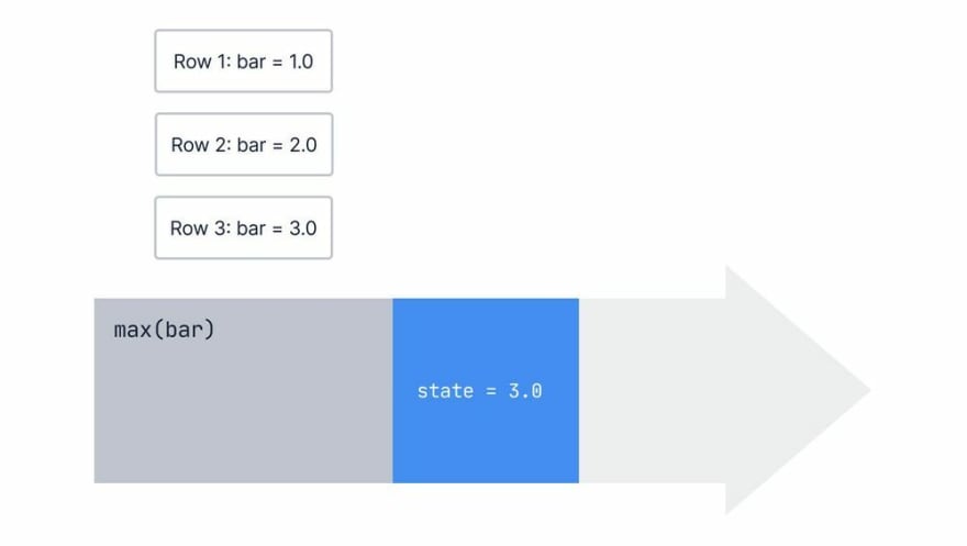
Finally, we don’t have any more rows to process, so we output our result:

So, to summarize, each row comes in, gets compared to our current state, and then the state gets updated to reflect the new greatest value. Then the next row comes in, and we repeat the process until we’ve processed all our rows and output the result.
 The max aggregate aggregation process, told in GIFs.
There’s a name for the function that processes each row and updates the internal state: the state transition function (or just “transition function” for short.) The transition function for an aggregate takes the current state and the value from the incoming row as arguments and produces a new state.
It’s defined like this, where current_value represents values from the incoming row, current_state represents the current aggregate state built up over the previous rows (or NULL if we haven’t yet gotten any), and next_state represents the output after analyzing the incoming row:
next_state = transition_func(current_state, current_value)
Aggregate internals: composite state
So, the max() aggregate has a straightforward state that contains just one value (the largest we’ve seen). But not all aggregates in PostgreSQL have such a simple state.
Let’s consider the aggregate for average (avg):
SELECT avg(bar) FROM foo;
To refresh, an average is defined as:
To calculate it, we store the sum and the count as our internal state and update our state as we process rows:
The `avg()` aggregation process, told in GIFs. For `avg()`, the transition function must update a more complex state since the sum and count are stored separately at each aggregation step.
But, when we’re ready to output our result for avg, we need to divide sum by count:
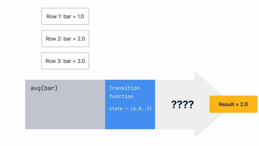 For some aggregates, we can output the state directly – but for others, we need to perform an operation on the state before calculating our final result.
There’s another function inside the aggregate that performs this calculation: the final function. Once we’ve processed all the rows, the final function takes the state and does whatever it needs to produce the result.
It’s defined like this, where final_state represents the output of the transition function after it has processed all the rows:
result = final_func(final_state)
And, through pictures:
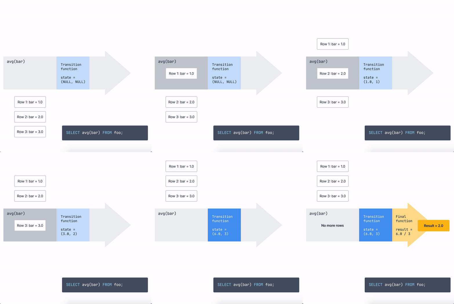 How the average aggregate works, told in GIFs. Here, we’re highlighting the role of the final function.
To summarize: as an aggregate scans over rows, its transition function updates its internal state. Once the aggregate has scanned all of the rows, its final function produces a result, which is returned to the user.
Improving the performance of aggregate functions
One interesting thing to note here: the transition function is called many, many more times than the final function: once for each row, whereas the final function is called once per group of rows.
Now, the transition function isn’t inherently more expensive than the final function on a per-call basis – but because there are usually orders of magnitude more rows going into the aggregate than coming out, the transition function step becomes the most expensive part very quickly. This is especially true when you have high volume time-series data being ingested at high rates; optimizing aggregate transition function calls is important for improving performance.
Luckily, PostgreSQL already has ways to optimize aggregates.
Parallelization and the combine function
Because the transition function is run on each row, some enterprising PostgreSQL developers asked: what if we parallelized the transition function calculation?
Let’s revisit our definitions for transition functions and final functions:
next_state = transition_func(current_state, current_value)
result = final_func(final_state)
We can run this in parallel by instantiating multiple copies of the transition function and handing a subset of rows to each instance. Then, each parallel aggregate will run the transition function over the subset of rows it sees, producing multiple (partial) states, one for each parallel aggregate. But, since we need to aggregate over the entire data set, we can’t run the final function on each parallel aggregate separately because they only have some of the rows.
So, now we’ve ended up in a bit of a pickle: we have multiple partial aggregate states, and the final function is only meant to work on the single, final state - right before we output the result to the user.
To solve this problem, we need a new type of function that takes two partial states and combines them into one so that the final function can do its work. This is (aptly) called the combine function.
We can run the combine function iteratively over all of the partial states that are created when we parallelize the aggregate.
combined_state = combine_func(partial_state_1, partial_state_2)
For instance, in avg, the combine function will add up the counts and sums.
 How parallel aggregation works, told in GIFs. Here, we’re highlighting the combine function (We’ve added a couple more rows to illustrate parallel aggregation.)
Then, after we have the combined state from all of our parallel aggregates, we run the final function and get our result.
Deduplication
Parallelization and the combine function are one way to reduce the cost of calling an aggregate, but it’s not the only way.
One other built-in PostgreSQL optimization that reduces an aggregate’s cost occurs in a statement like this:
SELECT avg(bar), avg(bar) / 2 AS half_avg FROM foo;
PostgreSQL will optimize this statement to evaluate the avg(bar) calculation only once and then use that result twice.
And, if we have different aggregates with the same transition function but different final functions? PostgreSQL further optimizes by calling the transition function (the expensive part) on all the rows and then doing both final functions! Pretty neat!
Now, that’s not all that PostgreSQL aggregates can do, but it’s a pretty good tour, and it’s enough to get us where we need to go today.
Two-step aggregation in TimescaleDB hyperfunctions
In TimescaleDB, we’ve implemented the two-step aggregation design pattern for our aggregate functions. This generalizes the PostgreSQL internal aggregation API and exposes it to the user via our aggregates, accessors, and rollup functions. (In other words, each of the internal PostgreSQL functions has an equivalent function in TimescaleDB hyperfunctions.)
As a refresher, when we talk about the two-step aggregation design pattern, we mean the following convention, where we have an inner aggregate call:

The inner aggregate call returns the internal state, just like the transition function does in PostgreSQL aggregates.
The outer accessor call takes the internal state and returns a result to the user, just like the final function does in PostgreSQL.
We also have special rollup functions defined for each of our aggregates that work much like PostgreSQL combine functions.
 PostgreSQL internal aggregation APIs and their TimescaleDB hyperfunctions’ equivalent
Why we use the two-step aggregate design pattern
There are four basic reasons we expose the two-step aggregate design pattern to users rather than leave it as an internal structure:
- Allow multi-parameter aggregates to re-use state, making them more efficient
- Cleanly distinguish between parameters that affect aggregates vs. accessors, making performance implications easier to understand and predict
- Enable easy to understand rollups, with logically consistent results, in continuous aggregates and window functions (one of our most common requests on continuous aggregates)
- Allow easier retrospective analysis of downsampled data in continuous aggregates as requirements change, but the data is already gone.
That’s a little theoretical, so let’s dive in and explain each one.
Re-using state
PostgreSQL is very good at optimizing statements (as we saw earlier in this post, through pictures ?), but you have to give it things in a way it can understand.
For instance, when we talked about deduplication, we saw that PostgreSQL could “figure out” when a statement occurs more than once in a query (i.e., avg(bar)) and only run the statement a single time to avoid redundant work:
SELECT avg(bar), avg(bar) / 2 AS half_avg FROM foo;
This works because the avg(bar) occurs multiple times without variation.
However, if I write the equation in a slightly different way and move the division inside the parentheses so that the expression avg(bar) doesn’t repeat so neatly, PostgreSQL can’t figure out how to optimize it:
SELECT avg(bar), avg(bar / 2) AS half_avg FROM foo;
It doesn’t know that the division is commutative, or that those two queries are equivalent.
This is a complicated problem for database developers to solve, and thus, as a PostgreSQL user, you need to make sure to write your query in a way that the database can understand.
Performance problems caused by equivalent statements that the database doesn’t understand are equal (or that are equal in the specific case you wrote, but not in the general case) can be some of the trickiest SQL optimizations to figure out as a user.
Therefore, when we design our APIs, we try to make it hard for users to unintentionally write low-performance code: in other words, the default option should be the high-performance option.
For the next bit, it’ll be useful to have a simple table defined as:
CREATE TABLE foo(
    ts timestamptz,
    val DOUBLE PRECISION);
Let’s look at an example of how we use two-step aggregation in the percentile approximation hyperfunction to allow PostgreSQL to optimize performance.
SELECT
    approx_percentile(0.1, percentile_agg(val)) as p10,
    approx_percentile(0.5, percentile_agg(val)) as p50,
    approx_percentile(0.9, percentile_agg(val)) as p90
FROM foo;
...is treated as the same as:
SELECT
    approx_percentile(0.1, pct_agg) as p10,
    approx_percentile(0.5, pct_agg) as p50,
    approx_percentile(0.9, pct_agg) as p90
FROM
(SELECT percentile_agg(val) as pct_agg FROM foo) pct;
This calling convention allows us to use identical aggregates so that, under the hood, PostgreSQL can deduplicate calls to the identical aggregates (and is faster as a result).
Now, let’s compare this to the one-step aggregate approach.
PostgreSQL can’t deduplicate aggregate calls here because the extra parameter in the approx_percentile aggregate changes with each call:
-- NB: THIS IS AN EXAMPLE OF AN API WE DECIDED NOT TO USE, IT DOES NOT WORK
SELECT
    approx_percentile(0.1, val) as p10,
    approx_percentile(0.5, val) as p50,
    approx_percentile(0.9, val) as p90
FROM foo;
So, even though all of those functions could use the same approximation built up over all the rows, PostgreSQL has no way of knowing that. The two-step aggregation approach enables us to structure our calls so that PostgreSQL can optimize our code, and it enables developers to understand when things will be more expensive and when they won't. Multiple different aggregates with different inputs will be expensive, whereas multiple accessors to the same aggregate will be much less expensive.
Cleanly distinguishing between aggregate/accessor parameters
We also chose the two-step aggregate approach because some of our aggregates can take multiple parameters or options themselves, and their accessors can also take options:
SELECT
    approx_percentile(0.5, uddsketch(1000, 0.001, val)) as median,--1000 buckets, 0.001 target err
    approx_percentile(0.9, uddsketch(1000, 0.001, val)) as p90,
    approx_percentile(0.5, uddsketch(100, 0.01, val)) as less_accurate_median -- modify the terms for the aggregate get a new approximation
FROM foo;
That’s an example of uddsketch, an advanced aggregation method for percentile approximation that can take its own parameters.
Imagine if the parameters were jumbled together in one aggregate:
-- NB: THIS IS AN EXAMPLE OF AN API WE DECIDED NOT TO USE, IT DOES NOT WORK
SELECT
    approx_percentile(0.5, 1000, 0.001, val) as median
FROM foo;
It’d be pretty difficult to understand which argument is related to which part of the functionality.
Conversely, the two-step approach separates the arguments to the accessor vs. aggregate very cleanly, where the aggregate function is defined in parenthesis within the inputs of our final function:
SELECT
    approx_percentile(0.5, uddsketch(1000, 0.001, val)) as median
FROM foo;
By making it clear which is which, users can know that if they change the inputs to the aggregate, they will get more (costly) aggregate nodes, =while inputs to the accessor are cheaper to change.
So, those are the first two reasons we expose the API - and what it allows developers to do as a result. The last two reasons involve continuous aggregates and how they relate to hyperfunctions, so first, a quick refresher on what they are.
Two-step aggregation + continuous aggregates in TimescaleDB
TimescaleDB includes a feature called continuous aggregates, which are designed to make queries on very large datasets run faster. TimescaleDB continuous aggregates continuously and incrementally store the results of an aggregation query in the background, so when you run the query, only the data that has changed needs to be computed, not the entire dataset.
In our discussion of the combine function above, we covered how you could take the expensive work of computing the transition function over every row and split the rows over multiple parallel aggregates to speed up the calculation.
TimescaleDB continuous aggregates do something similar, except they spread the computation work over time rather than between parallel processes running simultaneously. The continuous aggregate computes the transition function over a subset of rows inserted some time in the past, stores the result, and then, at query time, we only need to compute over the raw data for a small section of recent time that we haven’t yet calculated.
When we designed TimescaleDB hyperfunctions, we wanted them to work well within continuous aggregates and even open new possibilities for users.
Let’s say I create a continuous aggregate from the simple table above to compute the sum, average, and percentile (the latter using a hyperfunction) in 15 minute increments:
CREATE MATERIALIZED VIEW foo_15_min_agg
WITH (timescaledb.continuous)
AS SELECT id,
    time_bucket('15 min'::interval, ts) as bucket,
    sum(val),
    avg(val),
    percentile_agg(val)
FROM foo
GROUP BY id, time_bucket('15 min'::interval, ts);
And then what if I come back and I want to re-aggregate it to hours or days, rather than 15-minute buckets – or need to aggregate my data across all ids? Which aggregates can I do that for, and which can’t I?
Logically consistent rollups
One of the problems we wanted to solve with two-step aggregation was how to convey to the user when it is “okay” to re-aggregate and when it’s not. (By “okay,” I mean you would get the same result from the re-aggregated data as you would running the aggregate on the raw data directly.)
For instance:
SELECT sum(val) FROM tab;
-- is equivalent to:
SELECT sum(sum)
FROM
    (SELECT id, sum(val)
    FROM tab
    GROUP BY id) s;
But:
SELECT avg(val) FROM tab;
-- is NOT equivalent to:
SELECT avg(avg)
FROM
    (SELECT id, avg(val)
    FROM tab
    GROUP BY id) s;
Why is re-aggregation okay for sum but not for avg?
Technically, it’s logically consistent to re-aggregate when:
- The aggregate returns the internal aggregate state. The internal aggregate state for sum is
(sum), whereas for average, it is(sum, count). - The aggregate’s combine and transition functions are equivalent. For
sum(), the states and the operations are the same. Forcount(), the states are the same, but the transition and combine functions perform different operations on them.sum()’s transition function adds the incoming value to the state, and its combine function adds two states together, or a sum of sums. Conversely,count()s transition function increments the state for each incoming value, but its combine function adds two states together, or a sum of counts.
But, you have to have in-depth (and sometimes rather arcane) knowledge about each aggregate’s internals to know which ones meet the above criteria – and therefore, which ones you can re-aggregate.
With the two-step aggregate approach, we can convey when it is logically consistent to re-aggregate by exposing our equivalent of the combine function when the aggregate allows it.
We call that function rollup(). Rollup() takes multiple inputs from the aggregate and combines them into a single value.
All of our aggregates that can be combined have rollup functions that will combine the output of the aggregate from two different groups of rows. (Technically, rollup() is an aggregate function because it acts on multiple rows. For clarity, I’ll call them rollup functions to distinguish them from the base aggregate). Then you can call the accessor on the combined output!
So using that continuous aggregate we created to get a 1 day re-aggregation of our percentile_agg becomes as simple as:
SELECT id,
    time_bucket('1 day'::interval, bucket) as bucket,
    approx_percentile(0.5, rollup(percentile_agg)) as median
FROM foo_15_min_agg
GROUP BY id, time_bucket('1 day'::interval, bucket);
(We actually suggest that you create your continuous aggregates without calling the accessor function for this very reason. Then, you can just create views over top or put the accessor call in your query).
This brings us to our final reason.
Retrospective analysis using continuous aggregates
When we create a continuous aggregate, we’re defining a view of our data that we then could be stuck with for a very long time.
For example, we might have a data retention policy that deletes the underlying data after X time period. If we want to go back and re-calculate anything, it can be challenging, if not impossible, since we’ve “dropped” the data.
But, we understand that in the real world, you don’t always know what you’re going to need to analyze ahead of time.
Thus, we designed hyperfunctions to use the two-step aggregate approach, so they would better integrate with continuous aggregates. As a result, users store the aggregate state in the continuous aggregate view and modify accessor functions without requiring them to recalculate old states that might be difficult (or impossible) to reconstruct (because the data is archived, deleted, etc.).
The two-step aggregation design also allows for much greater flexibility with continuous aggregates. For instance, let’s take a continuous aggregate where we do the aggregate part of the two-step aggregation like this:
CREATE MATERIALIZED VIEW foo_15_min_agg
WITH (timescaledb.continuous)
AS SELECT id,
    time_bucket('15 min'::interval, ts) as bucket,
    percentile_agg(val)
FROM foo
GROUP BY id, time_bucket('15 min'::interval, ts);
When we first create the aggregate, we might only want to get the median:
SELECT
    approx_percentile(0.5, percentile_agg) as median
FROM foo_15_min_agg;
But then, later, we decide we want to know the 95th percentile as well.
Luckily, we don’t have to modify the continuous aggregate; we just modify the parameters to the accessor function in our original query to return the data we want from the aggregate state:
SELECT
    approx_percentile(0.5, percentile_agg) as median,
    approx_percentile(0.95, percentile_agg) as p95
FROM foo_15_min_agg;
And then, if a year later, we want the 99th percentile as well, we can do that too:
SELECT
    approx_percentile(0.5, percentile_agg) as median,
    approx_percentile(0.95, percentile_agg) as p95,
    approx_percentile(0.99, percentile_agg) as p99
FROM foo_15_min_agg;
That’s just scratching the surface. Ultimately, our goal is to provide a high level of developer productivity that enhances other PostgreSQL and TimescaleDB features, like aggregate deduplication and continuous aggregates.
An example of how the two-step aggregate design impacts hyperfunctions’ code
To illustrate how the two-step aggregate design pattern impacts how we think about and code hyperfunctions, let’s look at the time-weighted average family of functions. (Our what time-weighted averages are and why you should care post provides a lot of context for this next bit, so if you haven’t read it, we recommend doing so. You can also skip this next bit for now.)
The equation for the time-weighted average is as follows:
As we noted in the table above:
-
time_weight()is TimescaleDB hyperfunctions’ aggregate and corresponds to the transition function in PostgreSQL’s internal API. -
average()is the accessor, which corresponds to the PostgreSQL final function. -
rollup()for re-aggregation corresponds to the PostgreSQL combine function.
The time_weight() function returns an aggregate type that has to be usable by the other functions in the family.
In this case, we decided on a TimeWeightSummary type that is defined like so (in pseudocode):
TimeWeightSummary = (w_sum, first_pt, last_pt)
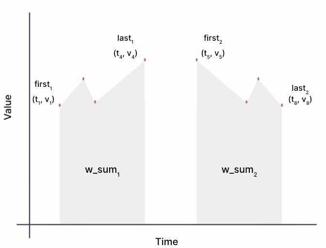
w_sum is the weighted sum (another name for the area under the curve), and first_pt and last_pt are the first and last (time, value) pairs in the rows that feed into the time_weight() aggregate.
Here’s a graphic depiction of those elements, which builds on our how to derive a time-weighted average theoretical description:
Depiction of the values we store in the `TimeWeightSummary` representation.
So, the time_weight() aggregate does all of the calculations as it receives each of the points in our graph and builds a weighted sum for the time period (ΔT) between the first and last points it “sees.” It then outputs the TimeWeightSummary.
The average() accessor function performs simple calculations to return the time-weighted average from the TimeWeightSummary (in pseudocode where pt.time() returns the time from the point):
func average(TimeWeightSummary tws)
-> float {
delta_t = tws.last_pt.time - tws.first_pt.time;
    time_weighted_average = tws.w_sum / delta_t;
return time_weighted_average;
}
But, as we built the time_weight hyperfunction, ensuring the rollup() function worked as expected was a little more difficult – and introduced constraints that impacted the design of our TimeWeightSummary data type.
To understand the rollup function, let’s use our graphical example and imagine the time_weight() function returns two TimeWeightSummaries from different regions of time like so:
The rollup() function needs to take in and return the same TimeWeightSummary data type so that our average() accessor can understand it. (This mirrors how PostgreSQL’s combine function takes in two states from the transition function and then returns a single state for the final function to process).
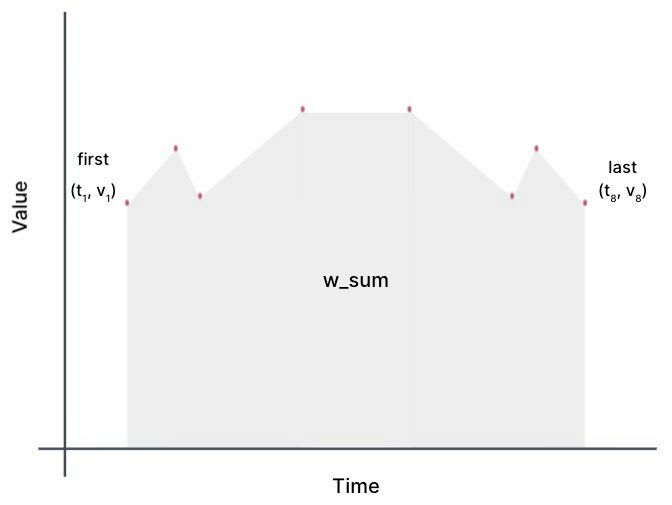
We also want the rollup() output to be the same as if we had computed the time_weight() over all the underlying data. The output should be a TimeWeightSummary representing the full region.
The TimeWeightSummary we output should also account for the area in the gap between these two weighted sum states:
 Mind the gap! (between one `TimeWeightSummary` and the next).
The gap area is easy to get because we have the last_1 and first_2 points - and it’s the same as the w_sum we’d get by running thetime_weight() aggregate on them.
Thus, the overall rollup() function needs to do something like this (where w_sum() extracts the weighted sum from the TimeWeightSummary):
func rollup(TimeWeightSummary tws1, TimeWeightSummary tws2)
-> TimeWeightSummary {
w_sum_gap = time_weight(tws1.last_pt, tws2.first_pt).w_sum;
w_sum_total = w_sum_gap + tws1.w_sum + tws2.w_sum;
return TimeWeightSummary(w_sum_total, tws1.first_pt, tws2.last_pt);
}
Graphically, that means we’d end up with a single TimeWeightSummary representing the whole area:
So that’s how the two-step aggregate design approach ends up affecting the real-world implementation of our time-weighted average hyperfunctions. The above explanations are a bit condensed, but they should give you a more concrete look at how time_weight() aggregate, average() accessor, and rollup() functions work.
Summing it up
Now that you’ve gotten a tour of the PostgreSQL aggregate API, how it inspired us to make the TimescaleDB hyperfunctions two-step aggregate API, and a few examples of how this works in practice, we hope you'll try it out yourself and tell us what you think :).
If you’d like to get started with hyperfunctions right away, spin up a fully managed TimescaleDB service and try it for free. Hyperfunctions are pre-loaded on each new database service on Timescale Forge, so after you create a new service, you’re all set to use them!
If you prefer to manage your own database instances, you can download and install the timescaledb_toolkit extension on GitHub, after which you’ll be able to use time_weight and all other hyperfunctions.
If you have questions or comments on this blog post, we’ve started a discussion on our GitHub page, and we’d love to hear from you. (And, if you like what you see, GitHub ⭐ are always welcome and appreciated too!)
We love building in public, and you can view our upcoming roadmap on GitHub for a list of proposed features, features we’re currently implementing, and features available to use today. For reference, the two-step aggregate approach isn’t just used in the stabilized hyperfunctions covered here; it’s also used in many of our experimental features, including:
-
stats_agg()uses two-step aggregation to make simple statistical aggregates, like average and standard deviation, easier to work with in continuous aggregates and to simplify computing rolling averages. -
counter_agg()uses two-step aggregation to make working with counters more efficient and composable. -
Hyperlogloguses two-step aggregation in conjunction with continuous aggregates to give users faster approximate COUNT DISTINCT rollups over longer periods of time.
These features will be stabilized soon, but we’d love your feedback while the APIs are still evolving. What would make them more intuitive? Easier to use? Open an issue or start a discussion!
This content originally appeared on DEV Community and was authored by davidkohn88
davidkohn88 | Sciencx (2021-08-30T09:04:30+00:00) How PostgreSQL aggregation works and how it inspired our hyperfunctions’ design. Retrieved from https://www.scien.cx/2021/08/30/how-postgresql-aggregation-works-and-how-it-inspired-our-hyperfunctions-design/
Please log in to upload a file.
There are no updates yet.
Click the Upload button above to add an update.


