This content originally appeared on DEV Community and was authored by Adnan Rahić
Don't you really hate latency?
Yeah, I hate it too.
Today, I want to talk about building applications on top of data warehouses. I want to discuss how to achieve low latency if your app is consuming data from BigQuery, Snowflake, Redshift, or any other cloud-based data warehouse.
My goal is to give you a crash course into data warehouse performance, explain how to understand the performance of data APIs and highlight a few tools that help build responsive apps on top of data warehouses.
What are Data Warehouses?
Broadly speaking, data warehouses are central locations for data from multiple sources. Call it a single source of truth. It's up to you to set up a process to extract, transform, and load (ETL) data from source systems based on a schedule or a set of events. Then you usually run reporting and data analysis to get some business insights.
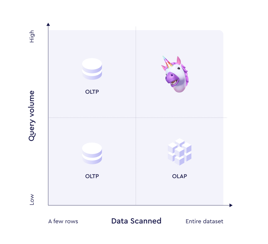
Data warehouses are usually optimized for online analytical processing (OLAP). It means running a relatively low volume of complex analytical queries with heavy joins of billion-row tables. The queries will often include numerical calculations using aggregate functions like AVG, COUNT DISTINCT, PERCENTILE_CONT, and many more like them.
As a direct consequence, data warehouses are often designed as auto-scaling and heavily distributed systems with columnar storage engines.
Snowflake Data Cloud, Google BigQuery, and Amazon Redshift are all good examples of such data warehouses and the most used and popular choice for storing huge amounts of data. If your company has a data warehouse in use, chances are it's one of these behemoths.
OLAP is often opposed to OLTP, which stands for online transaction processing. It means running a high volume of not-so-complex queries where the data is mostly inserted or updated rather than being read. However, the spectrum is much wider and there are more dimensions to it (pun intended).
As companies collect and transfer crazy volumes of data into their data warehouses, they want insight into this data. Your internal users become more interested in getting on-demand reports instead of weekly printouts. Your business becomes less tolerant of BI tools with time-to-insight comparable to how long it takes to make a cup of coffee rather than the time it takes to think about making one.
You, as an application developer, suddenly need to figure out how to build responsive and performant apps on top of data warehouses while keeping your business and users happy. But what exactly does "responsive and performant" mean? Let's figure that out.
Data Warehouse Performance from an App Developer's Perspective
As application developers, we'd like our users to maintain the feeling that they operate directly on the data regardless of an operation, data volume, or amount of other users acting in parallel. Studies say that an app reacts "instantaneously" if it responds to user actions within 10 ms, and 1 second is the limit above which an app risks interrupting their flow of thought. Here we come to query latency.
Latency
Query latency is the amount of time it takes to execute a query and receive the result.
Now let's take the speed of light into account! Seriously, let's imagine that a user from California sends a request to your app deployed in a popular region, e.g., us-east-1 on AWS. With the roundtrip of twice the distance of 3,000 miles and the speed of light of 186,000 mi/s, the minimum delay between sending the request and getting the response would be 30 ms. Wait, and what about our overseas users? You can actually use massively distributed CDNs like CloudFront or Netlify Edge to bring your app closer to users, but how practical is it for the data warehouses that your app interacts with?
It means that any request that your app makes to a data warehouse should take less than 1 second. Actually, way less than 1 second if we'd like to account for the speed of light, network delays, query execution time, time to run our business logic on top of the data, etc.
What affects the query execution time? Primarily, it's the amount of data that needs to be scanned. With larger datasets, these scans take more time. To distribute load, data warehouses use multiple nodes, which introduces delays for inter-node communications.
Now let's see what real-world data warehouses can offer.
Query Latency in BigQuery 🔍
Let's start with BigQuery, a serverless big data warehouse available as a part of the Google Cloud Platform. It's highly scalable, meaning that it can process tiny datasets as well as petabytes of data in seconds, using more cloud capacity as needed. You're able to manage its performance by choosing the pricing model (on-demand by default, flat-rate available as an option) which affects how BigQuery allocates slots, its virtual compute units with CPUs, memory, and temporary storage used to execute queries. BigQuery automatically calculates how many slots are required by each query, depending on query size and complexity. It's worth noting that every query competes for the slots with other queries within a GCP project, and also with other projects if you stick with the default on-demand pricing model as many do.
Let's use BigQuery's interactive console in GCP to estimate possible latencies.
After importing TPC-H data with 150 million rows into my own data set, I wanted to figure out a few sample queries I'd need for my analytics.
First of all, I'd want to see a list of all orders per day of certain status.
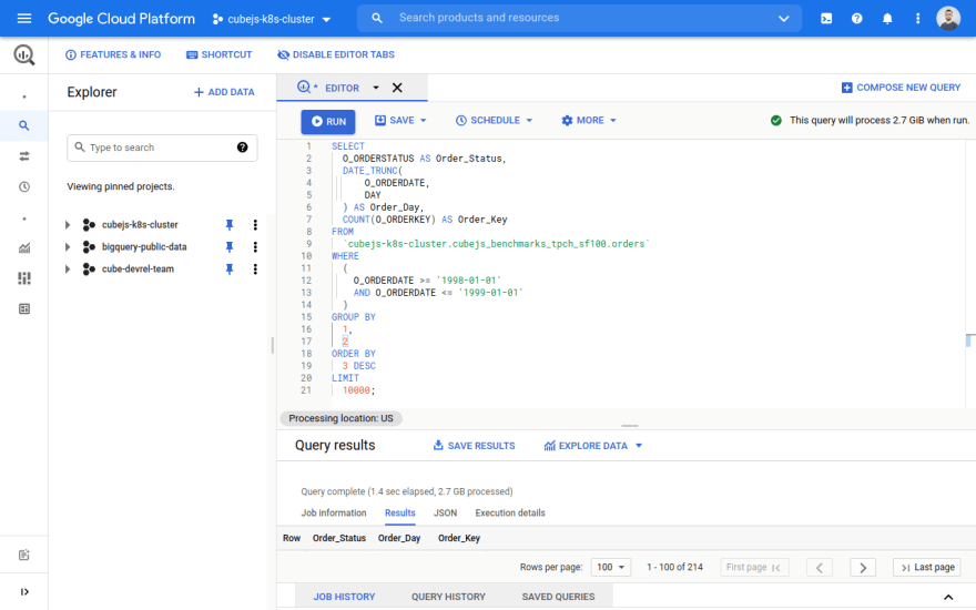
Here's the SQL query I ran in BigQuery.
The query takes 1.4 seconds to run, and it processed 2.7 GB. If you run it twice, you'll see that the second run latency is well under a second because the results of the first run were cached.
However, if you change the query, maybe add or update a filter in the WHERE clause, you'll still experience the same query latency of around a second and a half.
Why?
The answer is caching. BigQuery will cache the response of a query so the subsequent identical query gets a much quicker response time.
The BigQuery docs explain in more detail what cached results are. But, what you need to know is that to retrieve data from the cache, the duplicate query text must be exactly the same as the original query. All query results are cached in temporary tables for approximately 24 hours.
The pricing of cached queries is confusing. You are not charged for queries that use cached results, but these queries are subject to the BigQuery quota policies.
BigQuery is distributed by nature and its compute units are by default shared between users. That's why, in BigQuery, query latency includes not only query execution time but also initialization time which is spent to build a query plan, check quotas and limits, and allocate slots.
That's why it's unrealistic to expect BigQuery to provide sub-second query latency.
Okay, but what about Snowflake?
Query Latency in Snowflake ❄️
Unlike BigQuery, Snowflake doesn't share its compute resources between users. It processes queries using so-called virtual warehouses, and each virtual warehouse contains multiple dedicated compute nodes allocated from a cloud provider for your project. So, each virtual warehouse does not share compute resources with other virtual warehouses and has no impact on the performance of other virtual warehouses. However, your own queries will indeed compete for the resources of your virtual warehouses.
Snowflake’s query latency is improved by having pre-allocated virtual warehouses. However, everything comes at a price, pun intended.
Running a virtual warehouse will cost you something from 1 to 128 credits per hour. This ends up being between $50 and $6000 USD per day, according to Snowflake's usage-based pricing model.
Nobody likes to throw money down the drain for nothing, so Snowflake supports auto-suspending idle virtual warehouses after a specified amount of time. A suspended warehouse doesn't consume credits, but when a query comes, it should be re-provisioned.
Snowflake claims that warehouse provisioning generally takes 1 or 2 seconds, however, depending on the size of the warehouse and the availability of compute resources, it can take longer.
It means that with Snowflake we should either pay a significant premium or expect intermittent delays when a suspended virtual warehouse is being provisioned.
Let's use Snowflake's interactive console to check our intuition. I picked the TPC-H public dataset and used the built-in sample database provided by Snowflake. This data is provided in several schemas in the SNOWFLAKE_SAMPLE_DATA shared database, based on the exponent of 10, increasing from the base data set of around a few several million elements.
The schema I used is the TPCH_SF100 schema with 150 million rows.
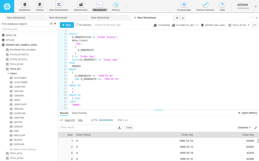
The data I want is an exact match for the query I ran against BigQuery in the example above. I want to see the total amount of orders grouped by day and status in a period between the years 1998 and 1999.
The query ran for 4.7 seconds. It returned 214 rows from a data set containing 150 million elements. I used the X-Small compute instance in Snowflake for this test. Of course, you can scale up the compute instances. But, how much money are you willing to spend?
So, it puts us in a world where getting a sub-second query latency from a data warehouse is something like a magic unicorn. 🦄
And I've only been talking about latency so far. We can all agree there are many more factors in play. Let me continue by explaining a few of them below.
Latency vs. Concurrency
As application developers, we build products used by hundreds, thousands, and millions of users. Rarely is it ever a lone user executing a single query at a given time. Your app should be able to run multiple queries against a data warehouse in parallel. The issue is that these queries will compete for available resources.
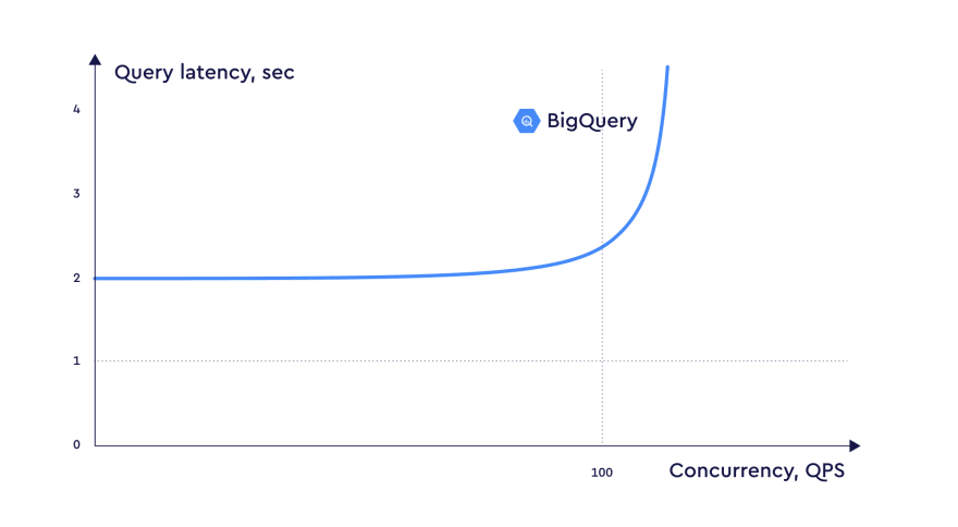
The question is, how would these parallel competing queries impact query latency? We know that BigQuery can provide an approximate 3 second response time for a query that processes vast amounts of data, possibly petabytes.
What would the response times be for 10 simultaneous queries? Or maybe, during Black Friday, even a few hundred queries?
Query concurrency is the amount of actively co-executing parallel queries. The "actively" part is important here because data warehouses can queue queries over a certain limit and run them only when previous queries are completed.
In BigQuery, according to its quotas and limits, concurrency is capped at 100 queries per project. That's a relatively high number, just beware of that "per project" part. It means that the quota is shared between all apps that interact with the same GCP project.
Queries with results that are returned from the query cache are also subject to the quota. The reason is that BigQuery needs to determine that it is a cache hit. However, you're not charged money for queries that use cached results.
Because BigQuery is such a black box, the best course of action is to improve query performance. Luckily, there's a detailed explanation in the BigQuery docs on how to achieve this. Here's a quick rundown.
You should limit the input data and data sources; the fewer bytes your query reads, the better. Never use SELECT * ... as it will scan all columns in the data set. Next, improve communication between slots, by reducing data before using a GROUP BY or JOIN clause.
Use ORDER BY and LIMIT only in the outermost query to improve the computation performance of queries and manage the query output. Remember, keeping the output bytes low is also important.
Because BigQuery is capped at 100 concurrent queries per project, using these best practices to improve query performance is definitely a must.
Snowflake is a bit different. It can use node sizes anywhere from 1 to 128 credits in a warehouse. Here's an explanation of how credits are charged. A warehouse can scale horizontally like a cluster if you select adding warehouses to a multi-cluster warehouse.
Resizing a warehouse can improve query performance, particularly for larger, more complex queries. However, warehouse resizing is not intended for handling concurrency issues; instead, use additional warehouses to handle the workload or use a multi-cluster warehouse.
Keep in mind that larger warehouses are not faster for smaller, more basic, queries. Small queries do not need a larger warehouse because they won’t benefit from the additional resources, regardless of the number of queries being processed concurrently. In general, you should try to match the size of the warehouse to the expected size and complexity of the queries to be processed by the warehouse.
So, if we expect multiple queries to run in parallel, we should research and be aware of query latency degradation that happens when the concurrency grows. Let's benchmark BigQuery to know for sure.
Latency vs. Concurrency in BigQuery
I decided to run a few load-test benchmarks with k6.io to measure the response-time percentile when querying BigQuery directly by using the SDK through a Node.js API. Here's the source code for the load tests. I decided to run a set of randomly generated queries.
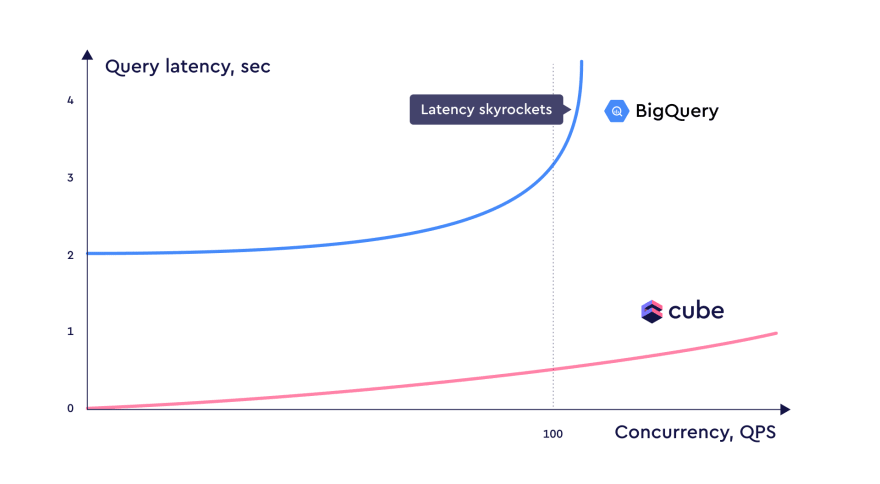
BigQuery is incredibly scalable and elastic, however, only up to 100 concurrent users.
First of all, I ran a benchmark with 1 concurrent user for 10 seconds. I can already see the percentile latency is unacceptable.
# 1 concurrent user

p(90)=2.51s
p(95)=2.58s
I then decided to run the same benchmark with 10 concurrent users for 10 seconds.
# 10 concurrent users

p(90)=2.31s
p(95)=2.41s
Then, a load test with 30 concurrent users.
# 30 concurrent users

p(90)=2.25s
p(95)=2.55s
As you can see the latency stays almost the same as BigQuery is autoscaling to handle the load.
It looks almost the same even with 100 concurrent users.
# 100 concurrent users

p(90)=2.16s
p(95)=2.4s
However, the issues pop up with more than 100 concurrent users. Request iterations started failing due to the concurrency limit.
High concurrency with sub-second latency 🦄
Here comes the real question. How to get acceptable latency with high concurrency? Does this unicorn even exist?
For this to become reality, you need materialized views. It's a set of pre-computed results from queries. You also need OLAP cubes.
Remember at the beginning of the article I mentioned OLAP? Well, here's why it's important. OLAP cubes are pre-computed multi-dimensional datasets. By using OLAP cubes you can filter a dataset by one or more dimensions and aggregate values along select dimensions.
By using materialized views with OLAP cubes, you can generate a condensed version of the source data by specifying attributes from the source itself.
This simple yet powerful optimization can reduce the size of the data set by several orders of magnitude, and ensures subsequent queries can be served by the same condensed data set if any matching attributes are found.
What is Cube?
Cube is an API server for making sense of huge datasets. It doesn't get any simpler than that. It's the de-facto Analytics API for Building Data Apps.
Why is Cube so cool? Let me tell you.
It's open-source with more than 11,000 stars on GitHub. Cube also integrates with every major database on the market today.
With Cube, you can create a semantic API layer on top of your data, manage access control, cache, and aggregate data. Cube is also visualization agnostic. It's up to you to use any front-end visualization library to build your own dashboards.
Building an Analytics API
I'll run a Cube instance to build the actual analytics API. It'll generate all the queries I need to run against BigQuery.
Note: Keep in mind you can set up Cube with any database of your choice, including Snowflake, Redshift, or any other data warehouse from the list here.
Configuring Cube with Docker Compose is the simplest way to get started.
Note: This example will run a single cube instance. For production, I recommend running multiple Cube instances. They include an API, a refresh worker, and Cube Store for caching. I'll talk about production-ready configs a bit further down in the article.
First up, create a new directory. Give it a name and make a docker-compose.yaml file. Copy this code into it.
version: '2.2'

services:
  cube:
    image: cubejs/cube:latest
    ports:
      - 4000:4000  # Cube.js API and Developer Playground
      - 3000:3000  # Dashboard app, if created
    environment:
      - CUBEJS_DEV_MODE=true

      - CUBEJS_DB_TYPE=bigquery
      - CUBEJS_DB_BQ_PROJECT_ID=your-project-id
      - CUBEJS_DB_BQ_KEY_FILE=/path/to/your/key.json

      - CUBEJS_API_SECRET=somesecret
    volumes:
      - .:/cube/conf
Configuring Access to BigQuery
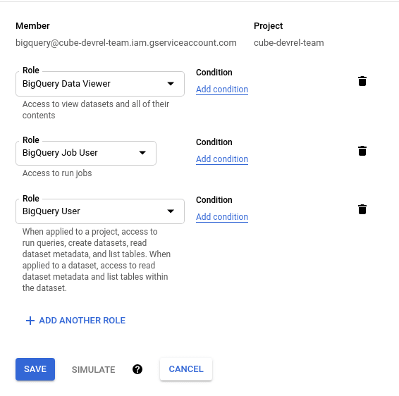
In my GCP account, I added a service account for accessing BigQuery. Here are the permissions I needed.
I then created a key for this service account and downloaded it to my local machine.
This means I can programmatically access this dataset once I start building my analytics API. Yes!
Make sure to set the CUBEJS_DB_TYPE to bigquery. The CUBEJS_DB_BQ_PROJECT_ID value should match the Project ID you created above. And the CUBEJS_DB_BQ_KEY_FILE is the JSON key you create for your Service Account.
What I tend to do is paste the key.json in the Cube directory. Referencing it in the docker-compose.yaml is simpler that way.
Next up, start Docker Compose. Open a terminal window in the Cube directory and run:
docker-compose up
This will start the Cube API server and the Developer Playground. The Playground is used to test queries, create schemas, generate SQL, and so much more. Open up localhost:4000 in your browser.
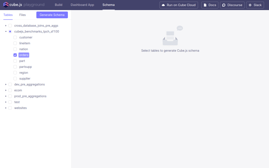
Navigate to the Schema page.
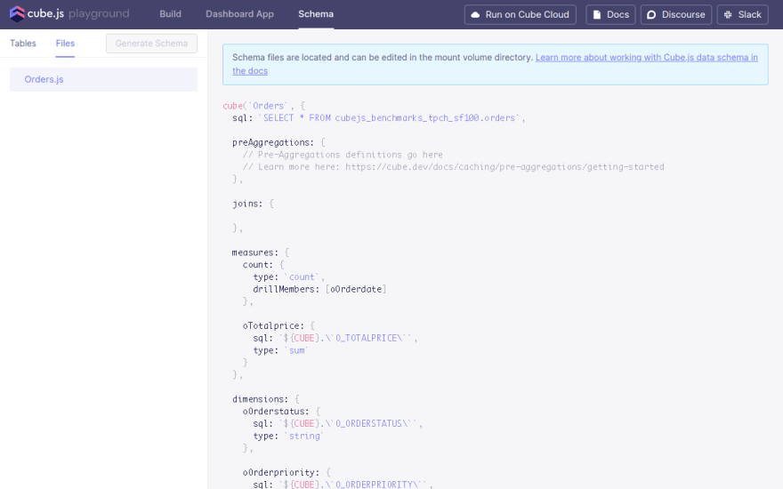
Here I generated a Schema from the orders table in the TPC-H data set. You'll see a file show up under Files.
This is the autogenerated Schema file that will contain measures and dimensions for all analytics values. I did need to edit a time dimension, however, to CAST() it to a TIMESTAMP.
oOrderdate: {
  sql: `CAST(${CUBE}.\`O_ORDERDATE\` AS TIMESTAMP)`,
  type: `time`
}
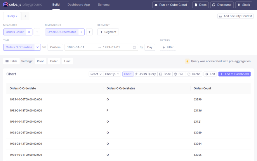
Next up, I ran the same query against the TPC-H data set through the Playground.
I get the same result set, which means the config works!
You can also see the generated SQL query.
I'm running this query without pre-aggregations, meaning it will almost take as long as querying BigQuery directly. This might be fine for testing but not for running in production.
There are two ways you can go about running Cube in production. First, you can use the hosted Cloud deployment of Cube. Or, run a production-ready setup yourself.
Pre-aggregations will cache your data and make it available for quicker querying. It's the bread and butter of Cube, and what makes it so powerful for building apps on top of Data Warehouses. I'll explain it in more detail in the section below.
Performance Improvement with Pre-Aggregations
In simple English, a pre-aggregation is a condensed version of source data. A pre-aggregation specifies attributes from the source, which Cube uses to condense the data. This optimization can reduce the size of the data set by several orders of magnitude, and ensures subsequent queries can be served by the same condensed data set if any matching attributes are found.
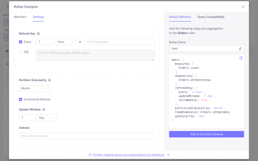
When you run a query in the Playground, you'll see a button show up called Query was not accelerated with pre-aggregation. Clicking on it opens this popup below.
This is a guide on how to enable a pre-aggregation for this query.
In the schema folder in my Cube app, I opened the Orders.js file and added this piece of code in the pre-aggregations block.
Note: The Orders.js file is located under the Schema tab in Cube Cloud.
cube(`Orders`, {
    ...

  preAggregations: {
    main: {
          measures: [
            Orders.count
          ],
          dimensions: [
            Orders.oOrderstatus
          ],
          refreshKey: {
            every: `1 hour`,
            updateWindow: `7 day`,
            incremental: true
          },
          partitionGranularity: `month`,
          timeDimension: Orders.oOrderdate,
          granularity: `day`
        }
  },

  ...
}
Here I specify what to pre-aggregate. I want a rollup on the count measure and the oOrderstatus dimension.
After adding the pre-aggregation, I ran the same query again.
This time it ran in under 200 ms. I consider this a win!
Raw Data Warehouse vs. Cube Performance Benchmarks
I ran a few load tests with k6.io to measure the response-time percentile differences between querying BigQuery directly by using the SDK through a Node.js API, versus using Cube through a Node.js API.
Here's the source code for the load tests. The tests themselves generate random queries that hit the database, with the sole purpose of avoiding the query cache. This will benchmark the raw performance of the database itself.
Let me remind you that with 30 concurrent users querying the BigQuery SDK for 10 seconds I see percentiles between 4 and 5 seconds, which is astonishingly far from ideal.
# 30 concurrent users
# BigQuery SDK

p(90)=2.25s
p(95)=2.55s
With Cube, I see percentiles around a half of a second with the same amount of concurrent users.
# 30 concurrent users
# Cube

p(90)=452.07ms
p(95)=660.03ms
However, I see a significant performance difference when running with more than 100 concurrent users.
# 100 concurrent users
# Cube

p(90)=598.92ms
p(95)=656.78ms
That's significantly quicker than it would take to query BigQuery directly with even one concurrent user.
Wrapping Up
In this blog post, I've tried making sense of data warehouse performance. I've also explored their theoretical and practical limits in terms of query latency and query concurrency.
You've learned how to find the magic unicorn of high concurrency and sub-second latency by creating an analytics API with Cube that adds a powerful caching layer on top of any data warehouse.
I hope you're now confident that it's possible to drop latency to below a second while getting a consistent concurrency of above 30 queries per second. The cool part is that the p(90) latency with Cube at 200 queries per second will stay below the p(90) latency of BigQuery at 30 queries per second.
I'd love to hear your feedback about these benchmarks in the Cube Community Slack. Click here to join!
Until next time, stay curious, and have fun coding. Also, feel free to leave Cube a ⭐ on GitHub if you liked this article. ✌️
This content originally appeared on DEV Community and was authored by Adnan Rahić
Adnan Rahić | Sciencx (2021-10-28T14:05:40+00:00) Performance capabilities of data warehouses and how Cube can help. Retrieved from https://www.scien.cx/2021/10/28/performance-capabilities-of-data-warehouses-and-how-cube-can-help/
Please log in to upload a file.
There are no updates yet.
Click the Upload button above to add an update.


