This content originally appeared on Level Up Coding - Medium and was authored by Gifari Hoque
HANDS-ON TUTORIALS / DATA CLEANING / STOCK MARKET
A Better Way to Handle Missing Values in your Dataset: Using IterativeImputer on the Stock Market Data (PART II)
Manipulating the historical stock market data with a multivariate imputer, the second part of this two-part series

Table of Contents
- Introduction
- IterativeImputer on the Stock Market Data
- Learning Your Military Time
- Manipulation
- The Results are in
- Understanding the Results - Conclusion
- References
- Final Words
Introduction
Welcome to the second part of this two-part series. In the first part, I went over several things including:
- Why you should care about missing data
- The different types of missing data (MCAR, MAR, & MNAR)
- Different ways to handle missing data (Univariate & Multivariate imputation)
I also went over how single imputation and multiple imputation methods affect the shape of the data distribution (skewness and kurtosis) with an example using the PIMA Indians Diabetes Database which can be found on Kaggle¹. If you’ve missed the first part, I highly encourage you to go ahead and check it out by clicking here! Without further ado, let’s get right into our second example.
IterativeImputer on the Stock Market Data
For this example, I’m going to be using the Stock Market data to show you how interesting IterativeImputer can be. I’ve made a notebook on Kaggle which simplifies this process down by using functions. I encourage you to play around with it after reading this. You can view/edit the notebook by clicking here.
Note:
Unfortunately, what may interest one, may not interest another.
- Just Another Law of Attraction by Gifari Hoque.
If you’re interested in more laws of attractions, leave a comment down below or reach out to me on any social media platform.
A little disclaimer before I dive deep into this example, because the stock market is being updated very often and because of how I’ll be manipulating the dataset (which you’ll see soon enough), we may never get the same results, and that’s completely fine!
I’ll be using the yfinance package to grab the historical market data for manipulation (of my own).
yfinance is a package used to download historical market data of stocks from Yahoo! Finance. It was developed by Ran Aroussi and is maintained by himself along with other contributors. To learn more about yfinance, click here to view the documentation on PyPi and click here to view the documentation on Ran Aroussi’s page. You can also see the source code on GitHub by clicking here.
You can install yfinance by running pip install yfinance or by downloading from PyPi, or by cloning/downloading from GitHub.
For this example, these are the necessary imports:
I chose to play around with Google’s data for this example.
The ticker symbol which I’ll be using is $GOOGL (Alphabet Inc Class A). I’ll be using data from the past 60 “stock market days” (period). I’m going to be using the closing price of every 30-minute interval.
NOTE:
- Some valid periods are: 1d,5d,1mo,3mo,6mo,1y,2y,5y,10y,ytd,max
- Some valid intervals are: 1m,2m,5m,15m,30m,60m,90m,1h,1d,5d,1wk,1mo,3mo
For this example, I advise you to only stick with intraday periods (1m,2m,5m,15m,30m,60m,90m, or 1h).
To learn more, please click here to read the yfinance documentation.
To download 30-minute interval data for $GOOGL for the past 60 days, run this code below:
You’ll then get a table like this after running the code above:
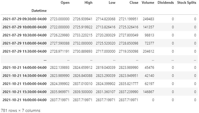
Without getting too much into detail, I’ll break this down. The Datetime index contains days from the past 60 market days (period) and goes by intervals of 30 minutes. 60 market days ago from when I’m writing this was July 29, 2021. The market opens at 09:30 AM and closes at 04:00 PM (eastern time zone). If you don’t yet know your military time, then pick it up, soldier.
Learning Your Military Time
Midnight (12:00:00 AM) is 00:00:00.
As soon as you hit 12:59:59 PM, instead of going down to 01:00:00 PM, you go to 13:00:00.
Keep going until it’s 23:59:59 which is 11:59:59 PM, and you’re back to midnight, at 00:00:00.
That’s right, military time is telling time without the use of AM or PM. I had to learn this the hard way 🤕.
If you’re still confused, here is a table that I’ve made for you:
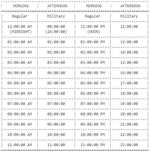
Okay, now going back to the dataframe, you can see that the first row’s Datetime is 09:30:30–04:00 and the very last row is 16:00:00–04:00. The market opens at 09:30 AM, closes at 04:00 PM. The “-04:00” part of each Datetime is saying that it’s based on New York’s time. The time zone in New York is “GMT-4” as of the day I’m writing this (this changes based on daylight saving).
The “Open” column is what price the stock was at exactly the corresponding time of the time specified in the row. The “High” and “Low” columns are the highest and lowest price that the stock reached within that 30-minute interval. The “Close” column is approximately what the price of the stock was at the very last second of the 30-minute interval. The “Volume” is pretty much the size of the trades within the interval.
For example, looking at the third row — 07/29/2021 at 10:30:00:
- At 10:30:00, the price per share of $GOOGL was approximately $2726.23 (“Open”).
- From 10:30:00 to 10:59:59, the lowest price each share became was $2720.28 (“Low”).
- The highest price each share became within that half-hour was $2733.22 (“High”).
- At 10:59:59, the price per share of $GOOGL was $2727.80 (“Close”).
Now that you have somewhat of an understanding of the layout of the data that we’ll be working with, now I’m going to explain more in depth what my motives are for this example. As stated before, I’m going to be using the 30-minute interval data, so this means that for every 30 minutes, I’ll have a price for $GOOGL, starting at 09:30:00 up until 16:00:00 (4 pm). I also decided to use the “Close” price of every interval instead of the “Open” price (except for the very first “Open” for each day — the price at 09:30:30). There’s no reason as to why I chose to do it this way, I just wanted to do it this way.
So this means, that I’ll have a price for $GOOGL for the following times: {09:30:00, 09:59:59, 10:29:59, 10:59:59, 11:29:59, 11:59:59, 12:29:59, 12:59:59, 13:29:59, 13:59:59, 14:29:59, 14:59:59, 15:29:59, and 15:59:59}. That’s right 14 different times for one day.
Note: The Stock Market occasionally closes earlier than 4pm eastern time.
I wanted to be able to group the data by dates, however, because the dates and times are all clumped together into one dataframe, I decided to convert this data into multiple individual dataframes (based on the date).
Every day is a new day, but every day has the same times. Therefore, every date will have 14 different time columns, in which there will be listed the price per share of $GOOGL at such specified date and time. Did I confuse you there? Here is how I wanted the layout will be:

Of course, this layout will be filled with values. For manipulation, I’ll replace random values in random columns with NaN, and then I’ll use IterativeImputer to try to guess what that number was. Sounds interesting yet?
Manipulation
Let’s now split the table up into individual tables based on the date and then extract the values we want from each table. Basically, each date will have its own dataframe.
The list dates is a list of all the dates, and the list data is a list of dataframes for each date.
These are the first ten dates in dates:
>>> dates[:10]
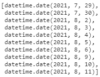
This is the data for the fifth date (08/04/2021) in data:
>>> data[4]
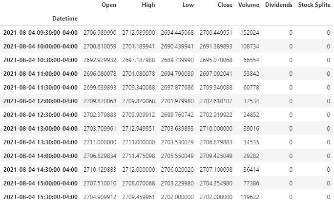
Now, let’s create a dictionary for our column names, append the values (rounded) and make a dataframe that will contain the “Open” price of each date at 09:30:00 and the “Close” price for each 30-minute interval for each day.
Notice that I’ve used “Open” and “Close” instead of “09:30:00” and “15:59:59”.
Note: Python’s built-in function round() can behave inappropriately. For instance, round(2.675, 2) gives 2.67. This isn’t a bug or an error, to learn more, click here. For my example, it doesn’t matter how round() treats the values.
Here is the sample code which will do the justice:
After you display adf.head(), you’ll get something like this:

Our new layout now has all the times listed in the column, and all the dates listed in the index. From here, let’s interpret this as a (date, time) pair. For example, (2021–08–04, 15:29:59) = 2704.35 means that on the date “2021–08–04” at the time “15:29:59”, the price of $GOOGL was $2704.35.
Now, len(adf) will return 60 (days), and adf.count().sum() will return 840 (60days * 14times = 840 values — prices).
Now let’s replace random values. For this demonstration, I’ll be using .sample() for random selection. Let’s randomly choose 8 different columns out of the 14, and of the 8 chosen columns, let’s choose 20% of the values at random and replace the values with NaN. This means that:
- 12 different rows (20% of 60 is 12) in 8 columns will be NaN
- 12 different days will have a missing price for the 8 chosen times
- We should expect to have a total of 12 * 8 = 96 values in total replaced with NaN, which means 744 values will not be NaN.
- Approximately 11.4286% of our dataset will now be NaN.
Now, if we run cdf.count().sum() , we’ll get 744.
These are the chosen columns (run cols to see yours):

If we run cdf.info(), we can see that 8 of the 14 columns now have 48 (out of 60) non-null values while the rest have 60 (out of 60) non-null values:
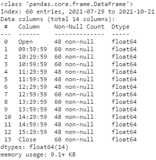
If you display cdf, you’ll realize that the rows chosen in one column are not the same as the rows chosen in another column. Here is a display of cdf.head():

Now let’s use Iterative Imputer to replace the NaNs! I’ll be using IterativeImputer() without any parameter changes for this example. Feel free to try out your own modifications on IterativeImputer().
I’ve created a dataframe of the transformed values and named the dataframe cdft. If we now check for any nulls in cdft, we’ll see that there aren’t any.
The Results are in
Now, for the final part, let’s compare the original value with the imputed value side by side, and see how close/far the imputer was to the original value. The code below may seem like it has a lot going on, but before I start explaining what my code does, my pictures (found below the code) are worth a thousand words each (I promise). Here is the code to see the results:
Before I confuse you any further, let my picture(s) explain to you the thousand words that I’ve promised:
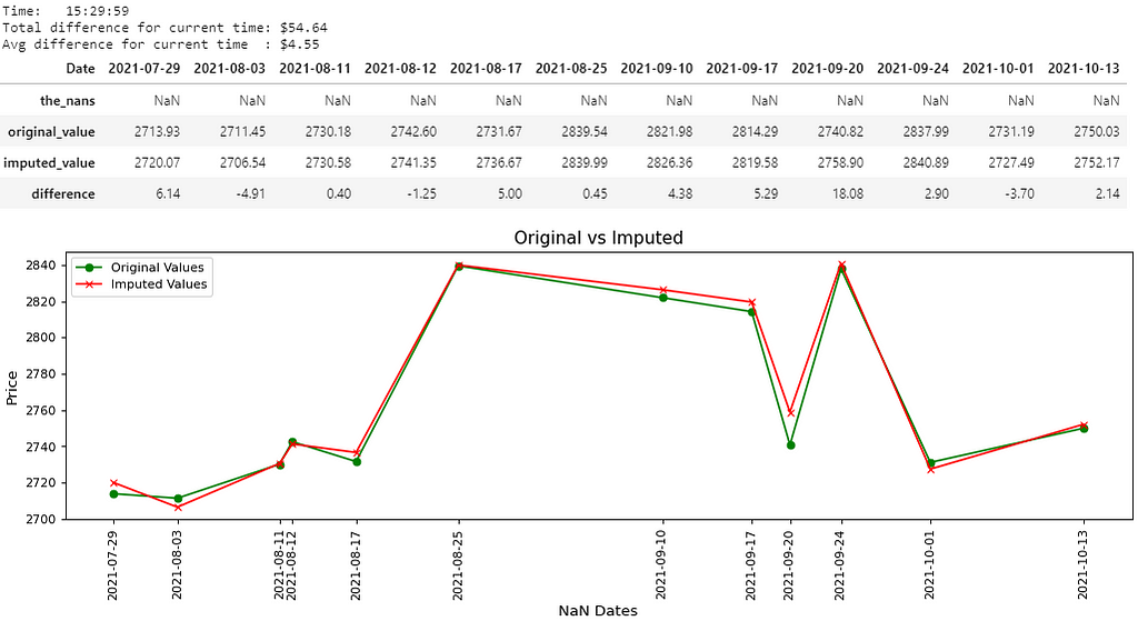
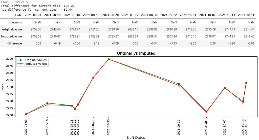
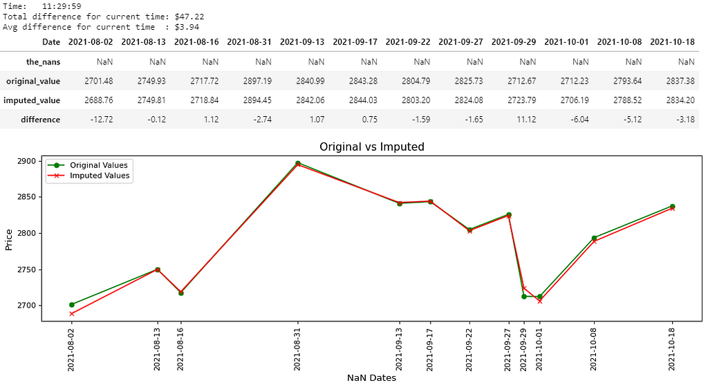
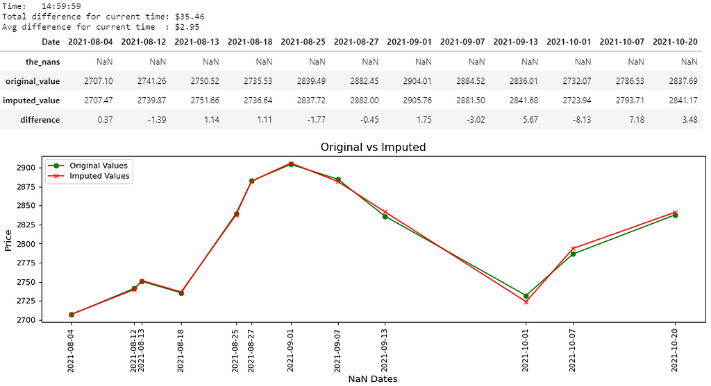
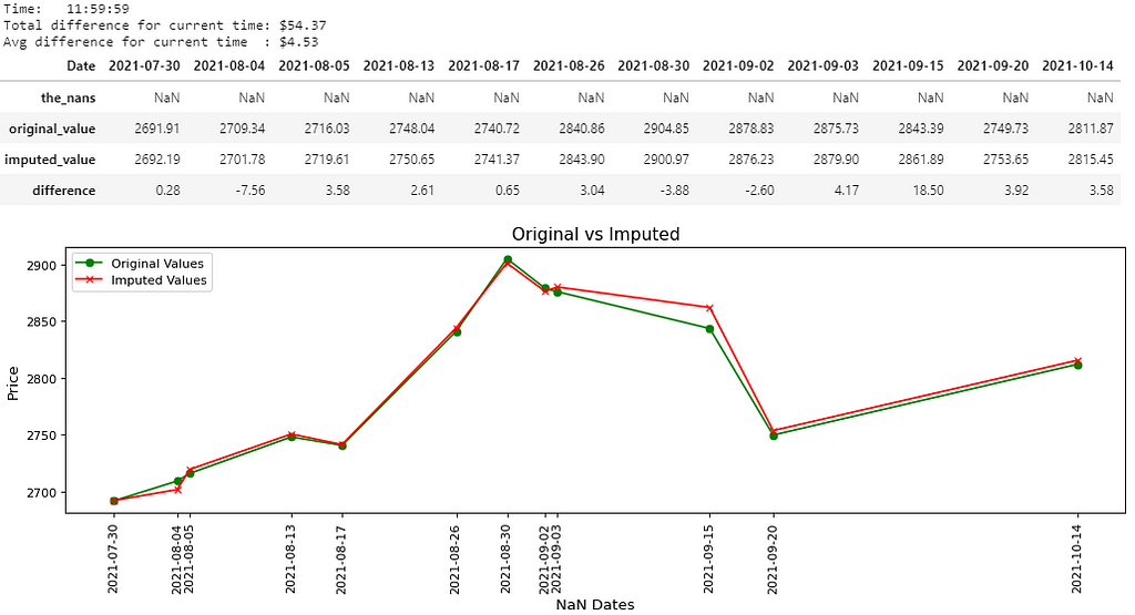
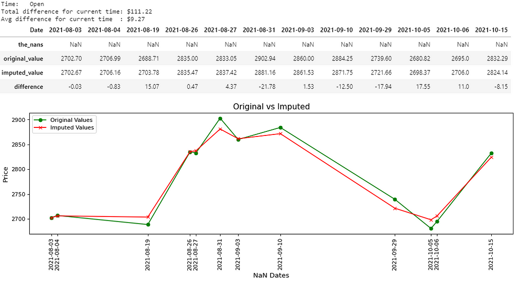
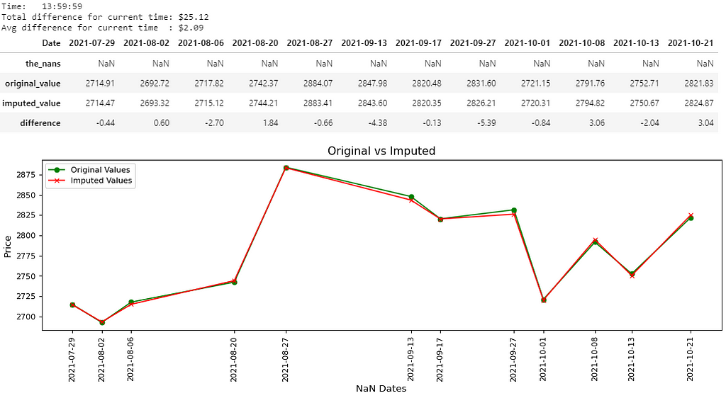
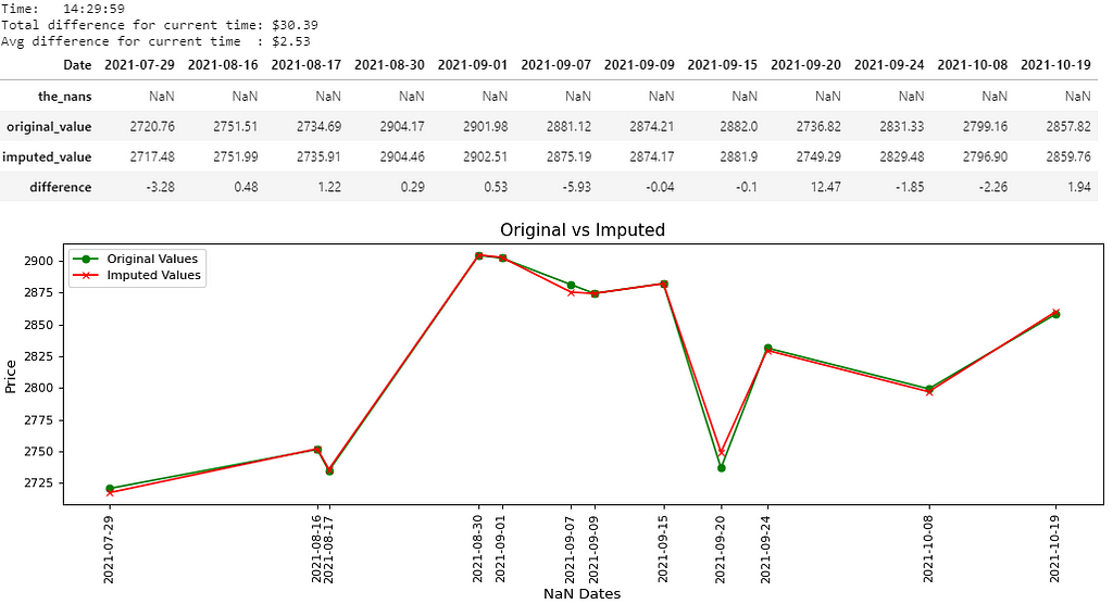

There you go, 8 pictures, so that must mean 8000 words, right? That’s probably the length of this notebook, and that’s not even counting the last picture. Maybe if the quality was better… Anyways, all jokes aside, I hope you guys are able to somewhat be able to see the values in the pictures above. I believe you guys can right-click each picture, open in a new tab and zoom in on it, nevertheless, I’ll write out the main results below:
- Picture 1 → (15:29:59); Difference: $54.64; Avg. Difference: $4.55
- Picture 2 → (12:29:59); Difference: $29.26; Avg. Difference: $2.44
- Picture 3 → (11:29:59); Difference: $47.22; Avg. Difference: $3.94
- Picture 4 → (14:59:59); Difference: $35.46; Avg. Difference: $2.95
- Picture 5 → (11:59:59); Difference: $54.37; Avg. Difference: $4.53
- Picture 6 → (Open); Difference: $111.22; Avg. Difference: $9.27
- Picture 7 → (13:59:59); Difference: $25.12; Avg. Difference: $2.09
- Picture 8 → (14:29:59); Difference: $30.39; Avg. Difference: $2.53
- Picture 9 → Overall Difference: $387.68;
Overall Average Difference: $4.04
Basically, what happened is, for easier comparison purposes, I’ve changed up the display of the dataframe.
For every “time” in cols, there will be a separate dataframe containing 4 rows, separate measurement variables currentDifference and currentAvg, and a separate graph. Only the (date, time) pair which were NaN will be shown in the results (including the graph).
There will also be two measurement variables in the end (as seen in picture 9) displaying the overallDifference and overallAvg.
The dataframe containing 4 rows will have a row for:
- Dataframe cdf (the_nans) → The (date, time) pair which was replaced with NaN. This should be a row of NaNs and nothing else.
- Dataframe adf (original_value) → The original value of the (date, time) pair.
- Dataframe cdft (imputed_value) → The imputed value of the (date, time) pair.
- Row 4 (difference) → The difference between the original value and the imputed value for that (date, time) pair.
- If the difference is negative, that means the imputer underestimated the original value by the displayed amount.
- If the difference is positive, that means the imputer overestimated the original value by the displayed amount.
currentDifference, overallDifference, currentAvg, and overallAvg are all used for measurement purposes:
- currentDifference → is the absolute value total of the difference row in the dataframe. Each “time” separation will have its own currentDifference.
- overallDifference → is all of the currentDifferencefrom each “time” separation, summed up. There is only one overallDifference which will be displayed in the end.
- currentAvg → is the average of the differences for the current “time”. This basically states that “for this current time, on an average, this is how far off the imputed values were from the original values.” Each “time” separation will have its own currentAvg.
- overallAvg → is the overall average of the differences. This basically states that “overall, on an average, this is how far off the imputed values were from the original values.” There is only one overallAvg which will be displayed in the end.
Understanding The Results
The overall average difference was $4.04. This may seem like a lot if we’re viewing this result as: “On an average, the imputations were $4.04 away from the actual value,” but we must not forget to consider the average price of $GOOGL from our values in our original dataframe adf.
adf.to_numpy().mean()
After running this code above, I get approximately $2788.45. This means that of the 840 prices in adf, the average price was $2788.45. If we divide the overall average difference by the average price:
4.04/2788.45 = 0.001448833581380337
That’s not anywhere even close to 1%. Investors wouldn’t even mind risking 1% of their portfolio.
Conclusion
I should mention again that in general, the multivariate approach is preferred over the univariate approach, but I personally think this depends on your own needs and goals for your project. In the first article, we saw the difference between a mean-imputation and iterative imputation using the PIMA Indians Diabetes Database, and in this article, we saw how close/far iterative imputed values were to the actual stock price. I have to say, even after using yfinance for this example, do play around with it and see what else you can do with it. It’s definitely a convenient way to obtain the stock market data.
I know that this was a long article, and I apologize for breaking it down into two separate parts, but I do hope that this was worth your time. This was my first article written on Medium, but as far as I can see, it won’t be my last. I hope you can make use of IterativeImputer, and I hope that you find at least one of my two examples to be useful.
Click on the link below to read the first part of this article:
A Better Way to Handle Missing Values in your Dataset: Using IterativeImputer (PART I)
Also, check out my notebook on Kaggle which includes the script for the stock price imputations using functions. After writing this article, I’ve decided to create this notebook. It’s pretty detailed, but if you use this article and the functions in this notebook, it hopefully makes your life easier.
Predict Missing Stock Prices with IterativeImputer
References
[1]: G. Hoque, A Better Way to Handle Missing Values in your Dataset: Using IterativeImputer (PART I) (2021), Medium (click to go back)
Final Words
If you notice any errors in my article, please do leave a comment and reach out to me so I can get it fixed ASAP! I don’t want to mislead anyone or teach anyone the wrong. To me, any criticism is positive criticism, that’s one of the best ways I learn. I’m also always open to tips and suggestions.
If you enjoyed reading this article, follow me on Medium and Kaggle where I’ll be posting more content from time to time. Also, feel free to connect with me on LinkedIn. If you think I deserve a coffee for my work, please do buy me one! Any support helps me keep going.
As always, thanks again for stopping by.
Disclaimer:
Nothing contained in this article should be construed as investment advice. I am by no means a financial advisor, nor do I plan to be one in the foreseeable future. If you think I should be a financial advisor, feel free to reach out to me.
A Better Way to Handle Missing Values in your Dataset: Using IterativeImputer on the Stock Market… was originally published in Level Up Coding on Medium, where people are continuing the conversation by highlighting and responding to this story.
This content originally appeared on Level Up Coding - Medium and was authored by Gifari Hoque
Gifari Hoque | Sciencx (2021-11-17T15:20:08+00:00) A Better Way to Handle Missing Values in your Dataset: Using IterativeImputer on the Stock Market…. Retrieved from https://www.scien.cx/2021/11/17/a-better-way-to-handle-missing-values-in-your-dataset-using-iterativeimputer-on-the-stock-market/
Please log in to upload a file.
There are no updates yet.
Click the Upload button above to add an update.
