This content originally appeared on Level Up Coding - Medium and was authored by Akash Raj
Variational Auto-Encoders are known to be susceptible to posterior collapse, where the approximate posterior collapses to the prior distribution due to the vanishing of the KL term (Bowman et al., 2015 [1]). This forces the approximate posterior to be independent of the data, i.e., q(z|x) = q(z) = p(z), where z represents the latent space, x represents the data, q(.) is the variational posterior and p(.) denotes the prior distribution. In this case, the recurrent decoder can heavily rely on the previous predicted output during training to decode the next item in the sequence. The latent representation of the input is ignored by the decoder and the z space does not learn any useful representation of the data.
To alleviate the issues posed by posterior collapse and the strong decoder, we explore (a) various approaches available and (b) introduce variants of existing approaches. We describe each of the approaches below. In the rest of this article, ELBO is used to refer to Evidence lower bound, RNN denotes Recurrent Neural Network.
1. KL Divergence Annealing
Following Bowman et al. (2015) [1], we can add a variable weight, λ to the KL term in the objective during training. At the start of training, we set λ = 0 and gradually increase it to a fixed threshold λₘ (which is a hyperparameter).

where t denotes the train step, r is the anneal rate and KLₑ𝒻𝒻. is the effective Kullback-Leibler divergence. In the beginning, this forces the model to encode as much information as possible from the latent space by learning to project the representation of the source sequence. The model potentially increases the mutual information between input and the latent space, I(x; z). As the training progresses, we let the model to regularize it with the KL cost. For the rate of increase, there are two choices, (a) linear increase, (b) exponential increase.
2. Free bits
The idea of free bits (FB) is to target a pre-specified rate (Alemi et al., 2017) [2]. Following Kingma et al. (2016) [3], we can use the following surrogate objective where K groups of stochastic units are encouraged to be used,

where r is pre-specified target rate and K denotes the latent dimension. Since the first r bits/nats of information is encoded for “free”, this technique is dubbed free bits. This technique offers an advantage over KL annealing since it is usually easy to determine the minimum number of bits and the number of stochastic units required to encode.
We note the following two problems in this method, (a) as long as the KL term is less than r, the actual ELBO is not being optimized, (b) ‘max’ introduces a discontinuity, i.e., it has a sharp transition at the boundary. To address these shortcomings Chen et al. (2016) [4] introduce soft free bits (SFB). Here the KL term is multiplied with a weight factor, 0 < β ≤ 1 which is adjusted by a factor α according to the target rate. While the optimization is smoother, this technique introduces many hyper parameters that need to be tuned. We use a modified version of free bits dubbed HA bits (initially introduced here: https://github.com/kastnerkyle/pytorch-text-vae) which compares the target rate with the mean of the KL terms over the entire layer.
3. Minimum Desired Rate
Minimum Desired Rate (MDR), proposed by Pelsmaeker and Aziz (2019) [5] is a technique that is used to attain ELBO values at a pre-specified rate of r. It has two advantages, (a) continuous gradients unlike Free Bits, and (b) fewer hyper parameters compared to Soft Free Bits. The ELBO is optimized subject to a minimum rate constraint r, i.e.,

where λ denotes variational parameters and θ denotes the parameters of the neural network. Note that for convenience, we derive the equations only for the supervised case, but is applicable to the unsupervised case as well. Since the above equation is intractable, we derive its Lagrangian dual function

We can use off-the-shelf stochastic gradient descent techniques with respect to u and stochastic gradient ascent with respect λ, θ.
4. Dropout
An advantage of using deep neural networks is their ability to learn complex and expressive relationship between the input and output. Despite their expressiveness and robustness, vanilla deep neural networks are prone to over-fitting which might lead to over confidence in wrong predictions. Several methods have been introduced in literature to address this issue: stopping the training when accuracy (performance) on the validation set starts to drop, introducing regularization terms such as L1 and L2 in the objective, and using the Bayesian framework in neural networks. Dropout is a technique that addresses the aforementioned problems of over-fitting and over-confidence. Dropout is used in encoder-decoder architectures to weaken the strong decoder. It forces the network to rely on the data representation in the latent space.
4.1 Random Dropout
We experiment with two variants of random dropout:
- Embedding Dropout: At each decoding time step, each unit in the embedding matrix is dropped out with a probability, p. We found that this did not help the model to utilize the latent space representations.
- Character Dropout: This technique introduced by Iyyer et al. (2015) [6], replaces random words in a sequence with the unknown word token, <UNK>. We adapt this technique by dropping a character at each decoding time step with a probability, β. Let dᵢ be an indicator variable sampled from a Bernoulli distribution, and dᵢ = 1 implies that iᵗʰ character is dropped. emb(xᵢ) represents the embedding of iᵗʰ word, xᵢ, then

In both the cases, the decoder is forced to use the representation of the latent space (which represents the lemma) and tag embedding information.

4.2 Contiguous dropout
This is an extension of the random character dropout procedure described previously. It involves 2 steps: (a) sample positions in a word sequence, (b) sample length for each position,

where mi is an indicator variable for the iᵗʰ position in the sequence chosen with probability β, lᵢ is the length sequence to drop from position i. We sample the length from a Poisson distribution with parameter λ. Figure above (B) shows an example of contiguous dropout. The top row shows the positions selected: m(3) and a(7). The Poisson distribution is then used to sample length at each of these positions (here sampled length is 3 for both the positions).
By using contiguous dropout, we encourage the latent space to learn n-gram features.
5. Independent hidden states — Historyless decoding
At each decoding step, the RNN decoder heavily relies on the previous observation. This prevents the network from using any useful information from the latent space, z. We can weaken the decoder by forcing it to ignore the history. This can be done in two ways:
- Semeniuta et al. (2017) [7] achieve historyless decoding by using using dropout on the input elements with dropout rate of 1.
- The RNN decoder is allowed to run for t time steps which generates t hidden states: [h₁ , h₂ , …, ht ]. From each hidden state, hᵢ, output character is generated independently.
Note that for both the approaches, at each time step we give the decoder (a) latent space information and (b) embedding. The two approaches are sometimes equivalent. In historyess decoding, we force the model to learn n-gram features.
6. Multi-task learning
Many of the aforementioned methods address the posterior collapse problem by weakening the decoder capacity to force the model to use latent information. This strategy is not ideal since it potentially degrades the quality of generated sequences. Kamoi and Fukutomi (2018) [8] propose a variant of VAE which utilizes multimodal prior and multi-task learning that generates well conditioned sequences without weakening the decoder.

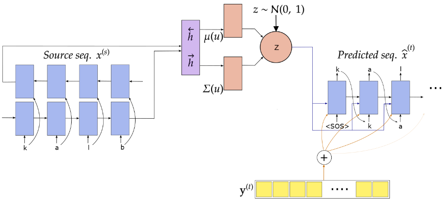
Pagliardini et al. (2017) report that the simple Bag-of-Words is effective at encoding the semantic content of a sentence. Following their work, in addition to the encoded sequence, we also input Bag-of-Characters features of the source sequence to the latent space. Figure above shows the architecture of the multi-task model.
Multi-task learning helps in acquiring better intermediate representations.
Experiments
We pick the task of Morphological reinflection. The task is to generate the target inflected sequence from a source inflected sequence and target morphological features. For training our model, we use the data from the shared task in SIGMORPHON 2016.

Above figure shows the overall model architecture for the supervised case. We use bi-directional Gated Recurrent Units for encoder and decoder. At each time step, we concatenate the forward and backward hidden states. The latent space is modeled with a Gaussian distribution z ∼N(μ(u), σ(u)), and u is the hidden representation of the source sequence. For details regarding the training procedure, refer to the repo.
Fixing a broken ELBO

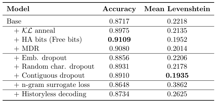
In the above table, we report accuracy (if the predicted sequence is equal to the ground truth target sequence) and mean Levenshtein distance (how far the predicted word is from the ground truth target sequence) when different methods to address posterior collapse are used. The Base model is the vanilla model without the modified ELBO. We observe that targeting the rate by using Free bits or MDR has the greatest increase in accuracy. Among the dropout schemes, random character dropout results in the best accuracy. However, we can see that Contiguous dropout has the smallest mean Levenshtein distance. It is our intuition that contiguous dropout forces the model to learn n-gram features which results in better predictions.

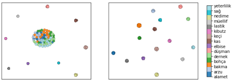
Above figure shows the tSNE plot of the latent space when (left) KL annealing is used and (right) MDR is used (words having the same lemma are colored similarly). MDR results in a more meaningful latent representation. In addition to getting a better latent representation, Free bits and MDR introduce hyperparameters which are more interpretable and practical than the weight factor in annealing.
Conclusion
In this article, we describe in brief, various methods to address the issue of posterior collapse. In addition, we introduce a few variants to existing methods. While some of the methods help alleviate the issue, they are dependent on the task at hand.
References
- Bowman, S. R., Vilnis, L., Vinyals, O., Dai, A. M., Jozefowicz, R., and Bengio, S. (2015). Generating sentences from a continuous space. arXiv preprint arXiv:1511.06349.
- Alemi, A. A., Poole, B., Fischer, I., Dillon, J. V., Saurous, R. A., and Murphy, K. (2017). Fixinga broken elbo.arXiv preprint arXiv:1711.00464.
- Kingma, D. P., Salimans, T., Jozefowicz, R., Chen, X., Sutskever, I., and Welling, M. (2016). Improved variational inference with inverse autoregressive flow. In Advances in neural information processing systems.
- Chen, X., Kingma, D. P., Salimans, T., Duan, Y., Dhariwal, P., Schulman, J., Sutskever, I., and Abbeel, P. (2016). Variational lossy autoencoder.arXiv preprint arXiv:1611.02731.
- Pelsmaeker, T. and Aziz, W. (2019). Effective estimation of deep generative language models.arXiv preprint arXiv:1904.08194.
- Iyyer, M., Manjunatha, V., Boyd-Graber, J., and Daum ́e III, H. (2015). Deep unordered composition rivals syntactic methods for text classification. In Proceedings of the 53rd Annual Meeting of the Association for Computational Linguistics and the 7th International Joint Conference on Natural Language Processing.
- Semeniuta, S., Severyn, A., and Barth, E. (2017). A hybrid convolutional variational autoencoder for text generation.arXiv preprint arXiv:1702.02390.
- Kamoi, R. and Fukutomi, H. (2018). Variational autoencoders for text modeling without weakening the decoder.
Posterior collapse and the strong generator problem was originally published in Level Up Coding on Medium, where people are continuing the conversation by highlighting and responding to this story.
This content originally appeared on Level Up Coding - Medium and was authored by Akash Raj
Akash Raj | Sciencx (2021-11-17T14:07:16+00:00) Posterior collapse and the strong generator problem. Retrieved from https://www.scien.cx/2021/11/17/posterior-collapse-and-the-strong-generator-problem/
Please log in to upload a file.
There are no updates yet.
Click the Upload button above to add an update.
