This content originally appeared on DEV Community and was authored by Mage
TLDR
Oftentimes when collecting consumer data, there are times when you’re unable to retrieve all the data. Instead of having a lack of data ruin your results, you’ll want to “guestimate” what the data should be.
Outline
Recap
Before we begin
What does impute mean?
3 ways to impute
Impute in Pandas
Next step
Recap
In the last section, we completed scaling categorical and numerical data so that all of our data is scaled properly. The higher ups want a list of past customers to target for our sales campaign, so we’re given new data that shows the history of how past customers interacted with our past 4 promotional emails.
 Big sales are coming soon!
Using the new data, our goal is to build a model for the remarketing campaign. There’s just one small problem. Code embedded in the marketing campaign email contained bugs, leaving us unable to identify what actions the people who clicked the email took. The bug occurs every 5 emails, but was patched by the 2nd wave of emails. In this section, we’ll go over imputing, a technique used to fill in unknown results.
 Bugs poke holes in my data (Source: Pest Control)
Before we begin
This guide will use the big_data dataset along with the new, promo dataset. It is recommended to read our guide on transforming data, using filters, and groups, to understand this section. Additionally, start reading from part 1, to understand all the different data types we’ll be working with and how we got to this point.
What does impute mean?
Impute is a technique used to fill in the missing information when given a dataset. When you impute, you use existing data to create references to missing data. Through imputing, data scientists are able to repair or patch parts of the data to give back its meaning. The quality of the data depends on how you handle imputing the data. The more complex a method is, the better the results. I’ll be showing 3 methods that are straightforward and easy for beginners, but do note that there are more out there that utilize other forms of AI, such as deep learning.
3 ways to impute
To get started, let’s think about what kind of references we can use in the data. The simplest and the most common method is by filling in the missing value with the value with the most occurences. Another method is by computing the average and storing the value there. Finally, the 3rd utilizes a mix of both methods, it checks the closest values to the term, then averages it.
Mean average value
Similarly, for mean average inputting, we calculate the average value out of all values in a column and then change the null values with the average value. Note that since this is an average, it will only work for numerical data and not categorical data, as categories are a classifier and not a count. In the case of a categorical variable, use a different method.
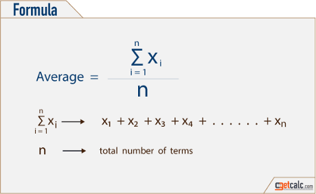 Take the sum and divide by the total (Source: getcalc)
Most frequent value
To calculate the most frequent value, first we search for the value that appears the most. Then we find all occurrences of the value and replace it with the most common value. A downside to this approach is that, since the value that is most common is used, it tends to skew data by adding bias towards the majority.
 The hand of bias tips the scales (Source: Global Government Forum)
K-Nearest Neighbors
K-Nearest Neighbors (KNN) is an algorithm that computes the closest “k” values in the graph. In imputation we’ll utilize this algorithm to determine a more accurate method that combines the best of both prior methods. Similar to taking the average, it takes into account portions of the dataset, but it only compares values nearby, resulting in less bias and more accuracy. Instead of repeating the most frequent value, it takes into consideration the other values, and constructs a graph to visit each neighborhood, or set of data points. However, since it is a brute force method that visits every value, it takes a long amount of time to run as the datasets grow larger.
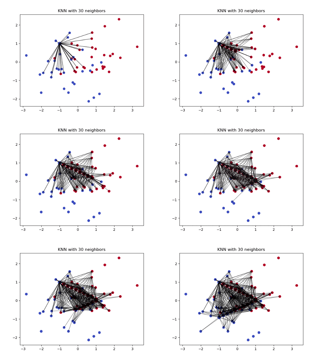 KNN graph (Source: Towards Data Science)
Impute in Pandas
First, we identify what type of data the promotional data we’re imputing is. By the looks of it, the value represents whether a user accepted the email campaign. In this case it’s a categorical variable, which represents the categories of “did accept” and “didn’t accept”.
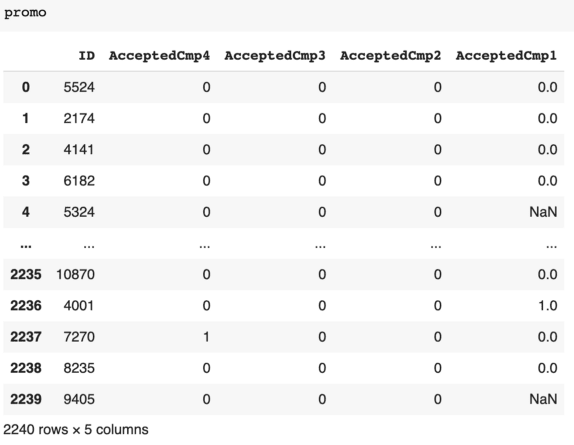
As a result, we cannot apply the mean average method and will use the most frequent value and K-nearest-neighbors to impute the AcceptedCmp1 in the promo dataset. Most frequent and mean average can be calculated using a SimpleImputer, but we’ll be using Pandas to show the basic steps taken.
Most frequent
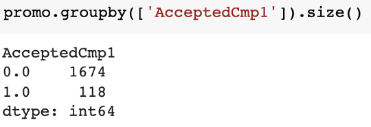
Using Pandas, along with grouping the values into True, False, and None, we can find the most frequently used of the 1s and 0s then set the NaN values to be equal. First, to find the count, we group the data to be 0 or 1 and take the count using size.

Next, we’ll use fillna to replace the values with 0. Previously, NaN couldn’t be an integer, so we also convert the float back to int, since true/false values should be 0 or 1.
![]()
Taking a look at the output, we now have this as our final dataset.

The breakdown can be found again by grouping and taking the size.
K-Nearest Neighbors
The algorithm of K-Nearest Neighbors is more complex and it visits each and every point. In this case, we’ll leverage the KNNImputer function from SciKit Learn.
Start by importing the functions we’ll be using, then select a value for “k”. This will determine the depth of the graph, and larger values will increase the time.
Since there are 2240 rows, we’ll pick a k value of 3 which is the floor of log(2240). I chose this arbitrarily by taking the log, since the function grows exponentially. Please note there may be better ways to determine the k value, which is better learned through trial and error.

Next, we can take our imputer, and apply it to our promo dataframe.
![]()
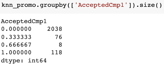 Upon inspection, we notice that some values aren’t exactly 1 or 0, but are in between.
We’ll take an extra step to round off, so “maybe” values become strictly “yes” or “no”.

Next Step
KNN was able to give more accurate results, but this doesn’t mean that the choices were correct. With such a big difference between accepted or not, using the most frequent value can save time compared to using the KNN. On the other hand, when you value accuracy and are dealing with smaller datasets or have a lot of time, KNNs will pick values in the middle of actual and frequent. Now that we’ve prepared all our data, we are now ready to begin training models. In the next series, we’ll look at how to train machine learning models for our remarketing use case. We’ll go deeper into what a model means, metrics, and answer the big question, which users should be part of the remarketing campaign?
This content originally appeared on DEV Community and was authored by Mage
Mage | Sciencx (2021-11-19T00:59:11+00:00) Guide to model training: Part 3 — Estimating your missing data. Retrieved from https://www.scien.cx/2021/11/19/guide-to-model-training-part-3-estimating-your-missing-data/
Please log in to upload a file.
There are no updates yet.
Click the Upload button above to add an update.

