This content originally appeared on Level Up Coding - Medium and was authored by Andrew Joseph Davies
Visualising the motion of two bodies due solely to their mutual gravitational attraction
Two masses represented in inertial space experience a mutual force of gravitational attraction.
The objective of the two-body problem is to determine how a pair of objects move relative to one another under the influence of gravity.
Review Example 2.2 in the latest Orbital Mechanics for Engineering Students textbook to understand the theory in depth.

Understanding the System
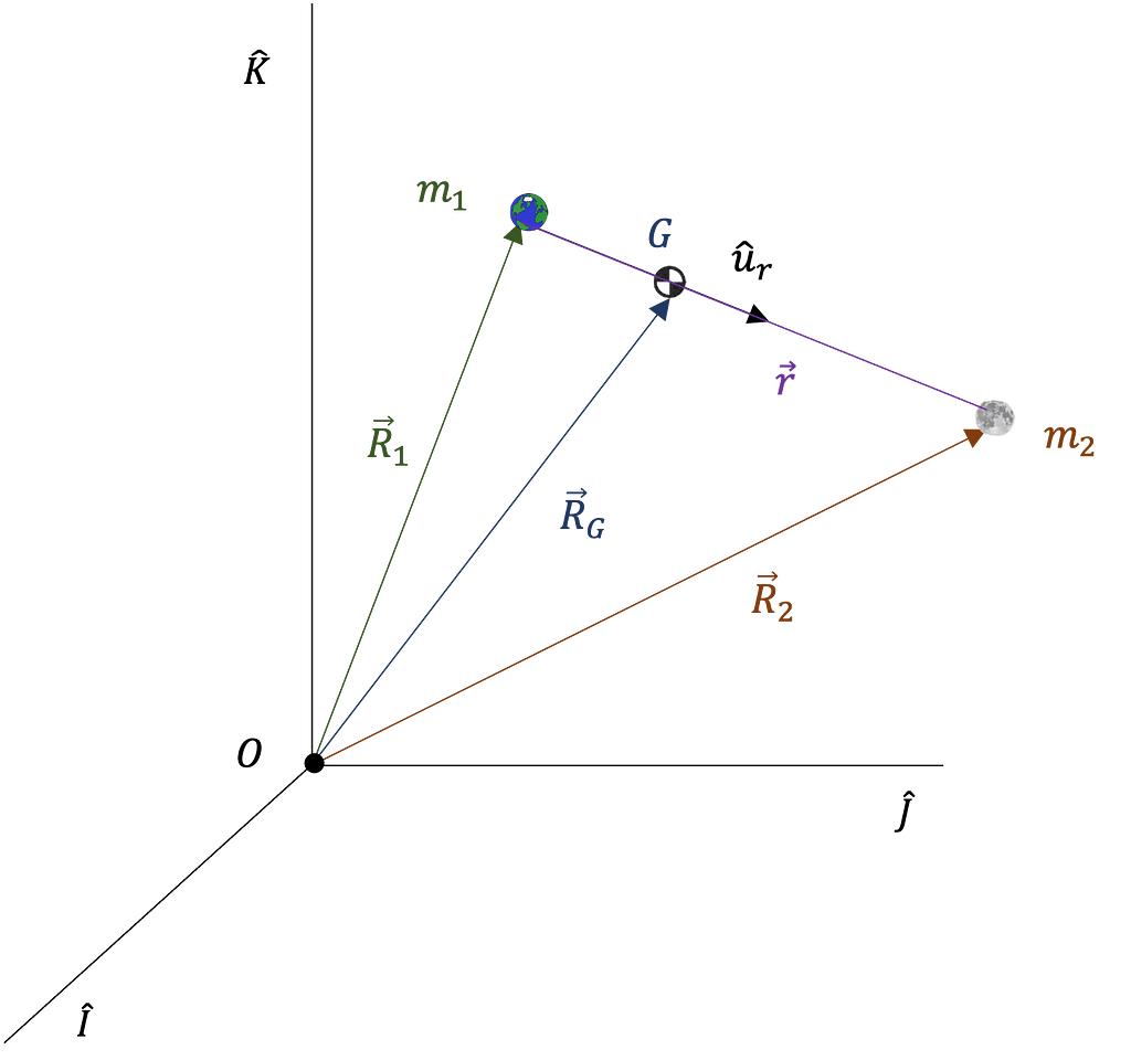
Figure 1 shows the two-body problem, a diagram of two masses m₁ and m₂ in an inertial reference frame. An inertial reference frame is essentially not accelerating. The system is free of external forces; only gravity acts between the two objects.
The critical parameters of interest from the diagram are:
- R₁: the position vector from the inertial frame origin to m1 as shown in Equation 1

- R₂: the position vector from the inertial frame origin to m2, given by Equation 2

- r: the position vector from m₁ to m₂, found using Equation 3

- G: the centre of mass of the system. If m₁ > m₂, the COM will lie closer to m₁.
- RG: the position vector from the inertial frame origin to the system’s centre of mass (COM) and is determined using Equation 4.

Deriving the Equations of Motion
Applying Newton’s Law of Universal Gravitation and Newton’s Second Law gives the equations of motion (EOM). Knowing the EOM and the initial position and velocity vectors makes it possible to propagate the system state through time.
Equation 5 is Newton’s Law of Universal Gravitation representing the force, F, of attraction between two particles of matter.

Equation 6 shows Newton’s second law stating the relationship between the acceleration of an object of matter and the sum of the forces acting it.

In the two-body system, the only force considered is gravity. Therefore, the force F₁₂ directed from m₁ to m₂ results from combining the above equation into the two-body EOM shown in Equation 7.

Newton’s third law indicates that the force directed from m₂ towards m₁ is equal and opposite to F₁₂. Equation 8 expresses the unit vector from object 1 to object 2.

Substituting the unit vector expression above into Equation 7 gives the final form of the equation of motion.

Equation 7 is a vector expression for acceleration with inertial components in the X, Y and Z directions. Thus, breaking Equations 9 and 10 into their constituent parts results in Equations 11— 16.

Numerical Integration
Numerically integrating the equations of motion gives the position and velocity of the masses over time. odeint from the scipy Python library is an adequate integral solver. The solver, such as Runge-Kutta, requires first-order ordinary differential equations (ODEs). Thus, several auxiliary variables facilitate the system modification, as shown in Equation 17–29.

The second-order system of six equations is cast to twelve first-order ODEs using the variables defined above, represented in Equations 30–41 below.
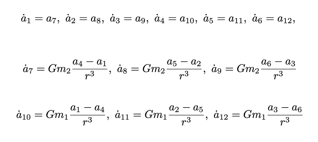
How is Numerical Integration Done Using Python
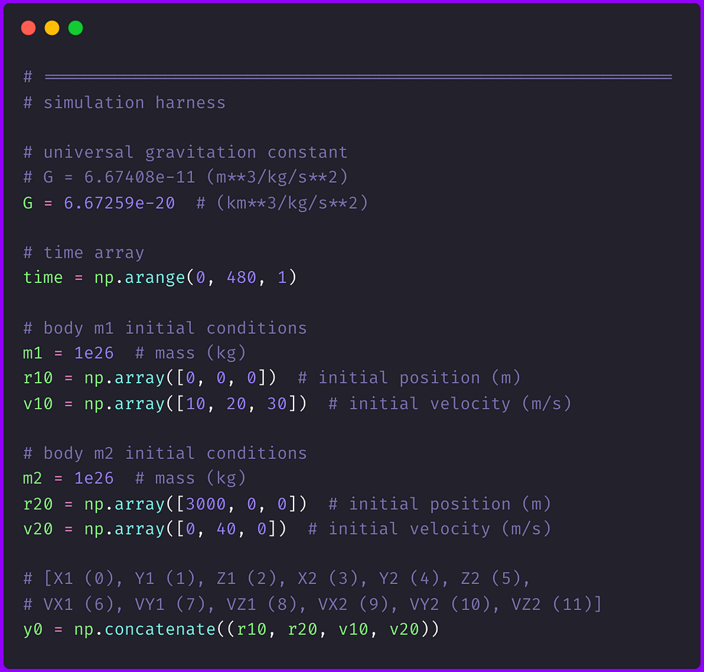
Initial conditions specify the positions and velocities of both objects at simulation commencement. Equations 42–45 show the conditions provided in the orbital mechanics textbook used in the simulation.

Python Implementation
Figure 2 shows the Python code defining the simulation harness parameters. These parameters include the mass of bodies 1 and 2 and the initial position and velocities in the state vector y₀.
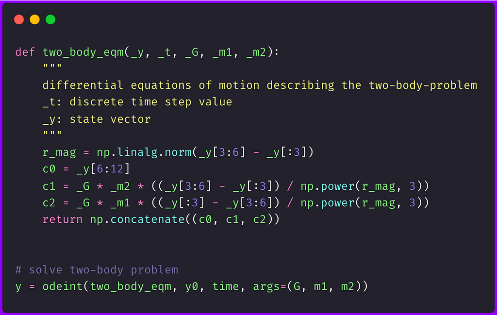
The two-body system of first-order ODEs is a Numpy array in Python, indicated by Figure 3. Verify that these equations match Equations 11 through 16.
Propagating the initial conditions through time to solve the two-body problem is performed using a single line of Python, as exhibited below.
# solve two-body problem
y = odeint(two_body_eqm, y0, time, args=(G, m1, m2))
y contains the history of the state vectors, position and velocities of m₁ and m₂, from time t₀ = 0 to t = 480 seconds.
- y[0:3]: the X, Y and Z components of R₁ at time tᵢ
- y[3:6]: the position of m₂ relative to the inertial frame
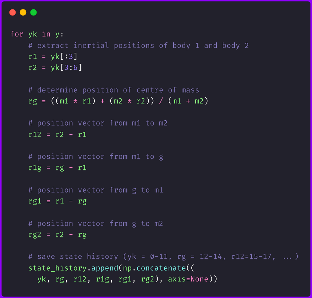
Figure 4 shows the Python code used to determine other position vectors relative to crucial points of interest, allowing motion visualisation from multiple perspectives, e.g. from the centre of mass or one of the objects.
Simulation Results
Figure 5(a) is the simulation animation from two perspectives.
- The trajectories of m₂ and the centre of mass as seen from body 1. Both the COM and body two appear to move in the shape of an ellipse.
- The orbits of both bodies that an observer would see positioned at the COM. Both orbits are elliptical.
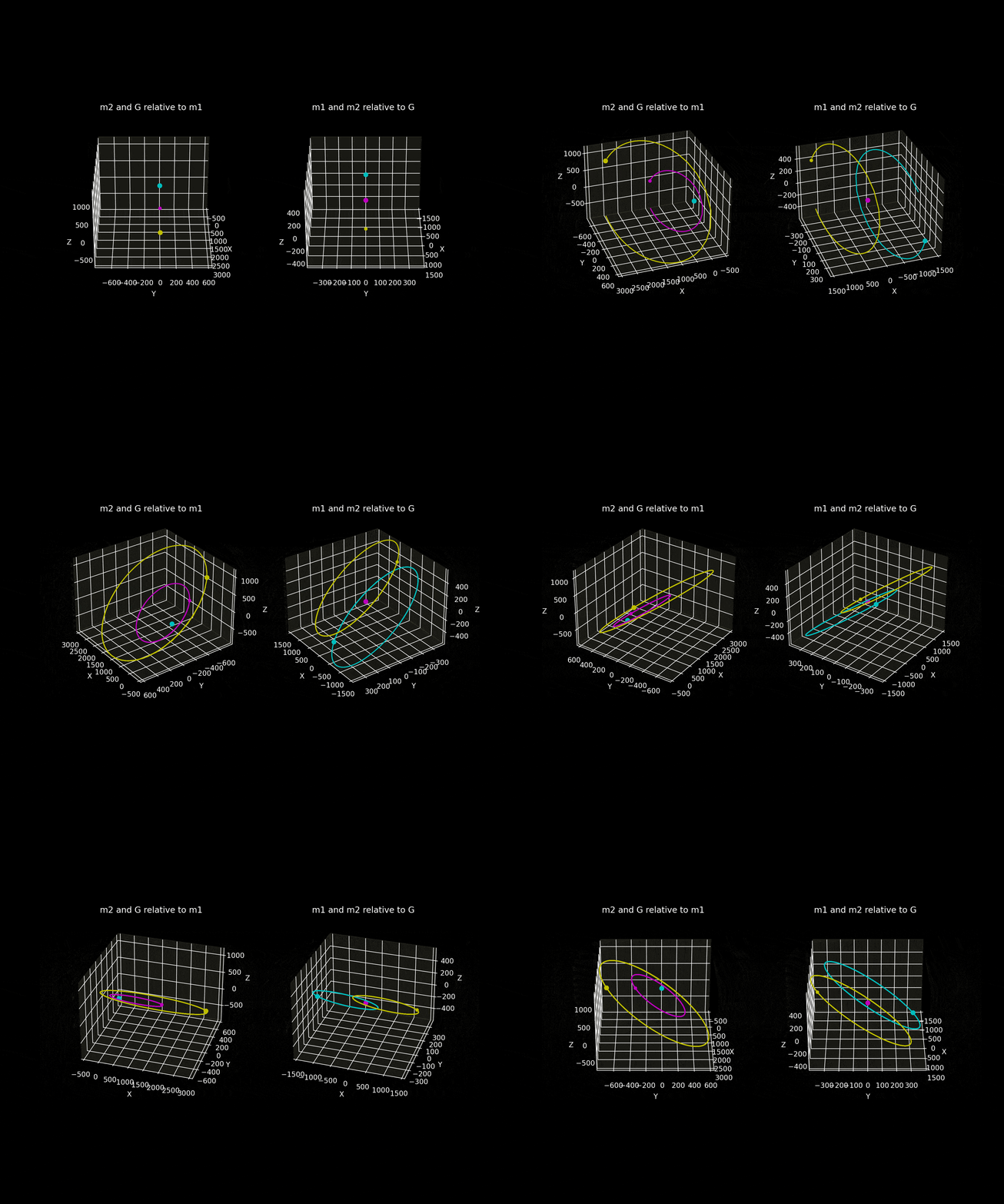
Figure 5b shows the motion of the two bodies relative to inertial space.
The two-body system establishes a periodic spiral motion around the straight-line trajectory of the entre of mass through space relative to the inertial frame.¹
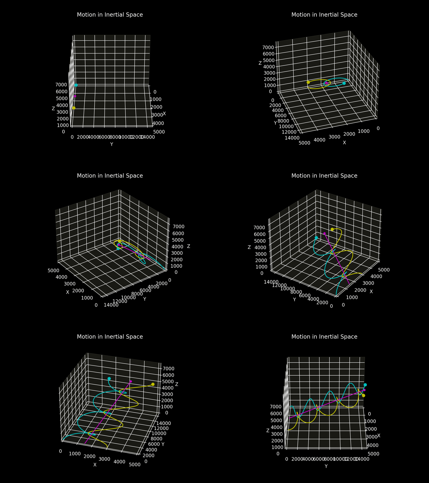
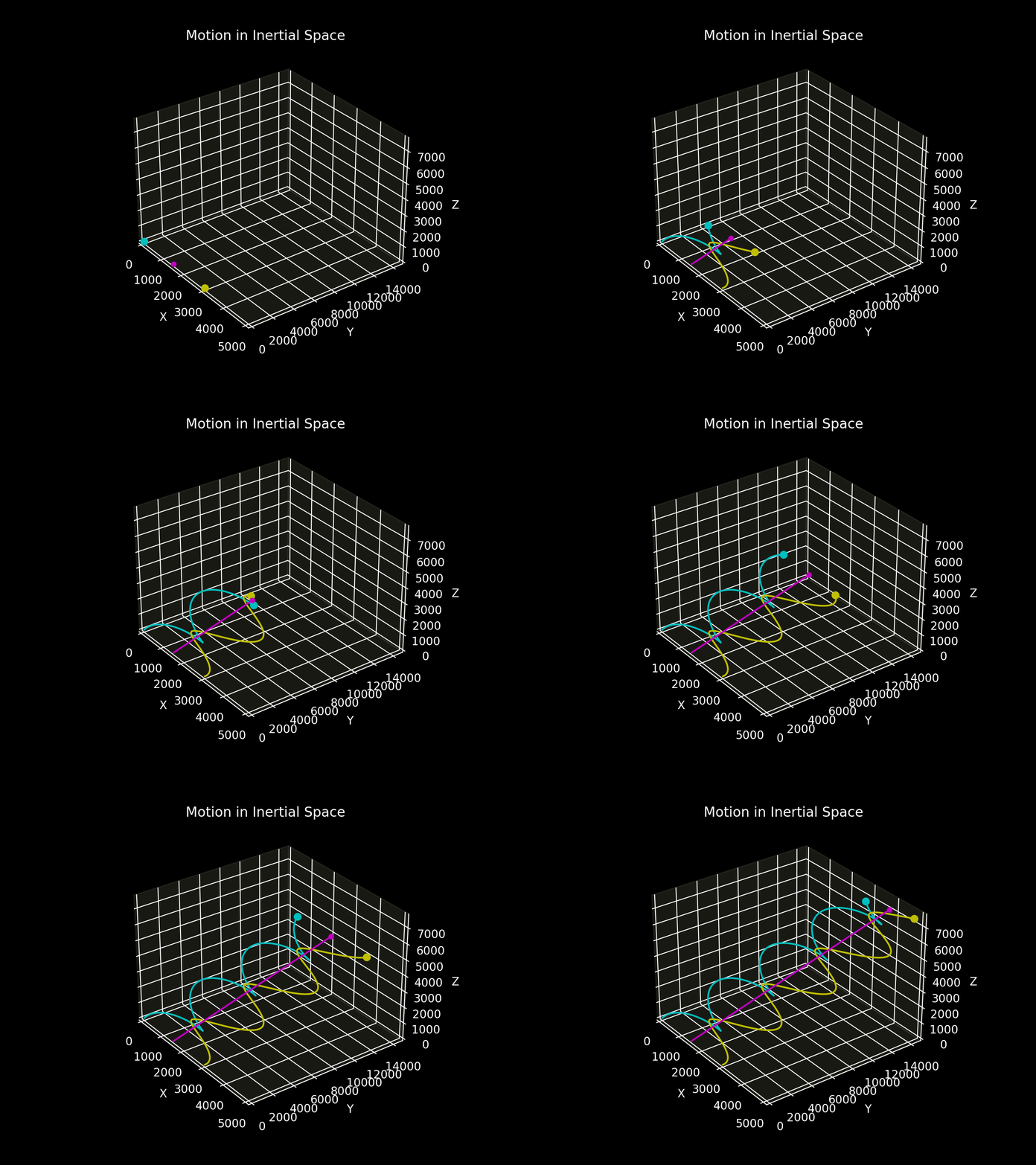
In the inertial frame, the centre of mass moves in a straight line with a constant velocity, proving that the system is free of external forces. This motion continues indefinitely.
This article demonstrates a method to find and then numerically integrate the equations of motion describing two bodies moving solely under the influence of the gravitational force acting between them.
The method presented to solve the two-body problem can simplify into a single body problem. See the references listed below for this analysis.
Similar Articles
3D Kinematics Visualisation with Python Libraries SymPy and NumPy
Find the Python code for solving the two-body equations of motion below.
References
[1] Orbital Mechanics for Engineering Students
- The process to simplify the Two-Body Problem to a single body problem.
The Two-Body Problem in Python was originally published in Level Up Coding on Medium, where people are continuing the conversation by highlighting and responding to this story.
This content originally appeared on Level Up Coding - Medium and was authored by Andrew Joseph Davies
Andrew Joseph Davies | Sciencx (2022-02-07T00:29:59+00:00) The Two-Body Problem in Python. Retrieved from https://www.scien.cx/2022/02/07/the-two-body-problem-in-python/
Please log in to upload a file.
There are no updates yet.
Click the Upload button above to add an update.
