How To Analyze Your WhatsApp Data With R Programming.

How To Analyze Your Whats App Data With R Programming.

Photo by Dima Solomin on Unsplash

In this post, I am going to analyze my departmental Whats app chat group Statistics Class of 2019. Thanks to a special package called rwhatsapp, this allows us to work with Whatsapp text data in R. We are also going to perform some text mining using the tidytext package.

#load libraries library(rwhatsapp) library(tidyverse) #load data chat <- rwa_read("C:/Users/Adejumo/Downloads/whatsapp.txt") %>% #remove messages without author 
filter(!is.na(author)) chat
Image by Author

I lost some messages, the messages are actually more than this. We have just 403 messages here.

Let’s see the number of messages sent on a daily basis.

chat %>% 
mutate(day = lubridate::date(time)) %>%
count(day) %>%
ggplot(aes(x = day, y = n)) +
geom_bar(stat = "identity") +
ylab("") +
xlab("") +
ggtitle("Messages per day")

Recently the group hasn’t been active as before.

The number of messages sent daily has dropped.

As of December, the maximum number of messages sent hasn’t been more than 20 messages per day. Seems everybody is busy with life (lol!). Let’s see the active members.

chat %>% 
mutate(day = lubridate::date(time)) %>%
count(author) %>%
arrange(desc(n)) %>%
head() %>%
ggplot(aes(x = reorder(author, n), y = n, fill = author)) + geom_bar(stat = "identity") +
ylab("") +
xlab("") +
coord_flip() +
ggtitle("Number of messages")

More than 90 messages have been sent by an unknown number.

Jagaban is the group admin, as expected of him, he is regularly active.

Let’s get to the fun part, lets see the most often used emojis in the group.

library("ggimage") emoji_data <- 
rwhatsapp::emojis %>% # data built into package mutate(hex_runes1 = gsub("\\s.*", "", hex_runes)) %>% # ignore combined emojis mutate(emoji_url = paste0("https://abs.twimg.com/emoji/v2/72x72/", tolower(hex_runes1), ".png"))
chat %>% 
unnest(emoji) %>%
count(author, emoji, sort = TRUE) %>%
arrange(desc(n)) %>% head(10) %>%
group_by(author) %>%
left_join(emoji_data, by = "emoji") %>%
ggplot(aes(x = reorder(emoji, n), y = n, fill = author)) + geom_col(show.legend = FALSE) +
ylab("") + xlab("") +
coord_flip() +
geom_image(aes(y = n + 20, image = emoji_url)) +
facet_wrap(~author, ncol = 2, scales = "free_y") +
ggtitle("Most often used emojis") +
theme(axis.text.y = element_blank(), axis.ticks.y = element_blank())

Looks like the most popular emoji is the face with tears of joy. The group admin Jagaban is also the member that sends the most emoji. Let’s compare favorite words.

library(tidytext) 
chat %>%
unnest_tokens(input = text, output = word) %>%
count(author, word, sort = TRUE) %>%
head(80) %>%
group_by(author) %>%
top_n(n = 6, n) %>%
ggplot(aes(x = reorder_within(word, n, author), y = n, fill = author)) +
geom_col(show.legend = FALSE) +
ylab("") +
xlab("") +
coord_flip() +
facet_wrap(~author, ncol = 2, scales = "free_y") + scale_x_reordered() +
ggtitle("Most often used words")

First of all, we have to do is remove the words “media” and “omitted”, these are placeholders Whats app puts into the log file instead of pictures or video.

There are other words that don’t look particularly useful either, these words are called stopwords: words that don’t carry substantial meaning e.g, and, or, and so on. There are some pidgin words also that need to be removed such as dey, na, and so on.

Pidgin words are slang used in Nigeria, if you have been to Nigeria before you will know what I am talking about.

library("stopwords") 
to_remove <- c(stopwords(language = "en"), "media","omitted","na","2","s","u","ahni","irc","dey","3","au","mak","u","don","naa","4","6","una","b","oo","2021","go","sir") chat %>% unnest_tokens(input = text, output = word) %>% 
filter(!word %in% to_remove) %>%
count(author, word, sort = TRUE) %>%
head(90) %>% group_by(author) %>%
top_n(n = 6, n) %>%
ggplot(aes(x = reorder_within(word, n, author), y = n, fill = author)) +
geom_col(show.legend = FALSE) + ylab("") +
xlab("") +
coord_flip() +
facet_wrap(~author, ncol = 2, scales = "free_y") + scale_x_reordered() + ggtitle("Most often used words")

The unknown number sends more links which are mostly job links from the link name ngojobsite.com in the group chat.

Another text mining technique we can do is to calculate lexical diversity. This allows us to see how many unique words are used by an author.

chat %>% 
unnest_tokens(input = text, output = word) %>%
filter(!word %in% to_remove) %>%
count(author, word, sort = TRUE) %>%
group_by(author) %>%
summarise(lex_diversity = n_distinct(word)) %>% arrange(desc(lex_diversity)) %>%
head(10) %>%
ggplot(aes(x = reorder(author, lex_diversity), y = lex_diversity, fill = author)) +
geom_col(show.legend = FALSE) +
scale_y_continuous(expand = (mult = c(0, 0, 0, 500))) + geom_text(aes(label = scales::comma(lex_diversity)), hjust = -0.1) + ylab("unique words") +
xlab("") +
ggtitle("Lexical Diversity") +
coord_flip()

From previous plots, we know that the unknown number mostly shares website links.

Let’s see what the unique words used by Limitless who is the second on the list.

o_words <- chat %>% 
unnest_tokens(input = text, output = word) %>%
filter(author != "Limitless") %>%
count(word, sort = TRUE) chat %>%
unnest_tokens(input = text, output = word) %>%
filter(author == "Limitless") %>%
count(word, sort = TRUE) %>%
filter(!word %in% o_words$word) %>% # only select words nobody else uses top_n(n = 6, n) %>%
ggplot(aes(x = reorder(word, n), y = n, fill = word)) + geom_col(show.legend = FALSE) +
ylab("") +
xlab("") +
coord_flip() +
ggtitle("Unique words of Limitless")

Seeing from the above, these are words that are unique to Limitless.

You can perform a similar analysis on your data and even do better.

Originally published at https://www.adejumoridwan.com on January 16, 2022.

Level Up Coding

Thanks for being a part of our community! Before you go:

🚀👉 Join the Level Up talent collective and find an amazing job


How To Analyze Your WhatsApp Data With R Programming. was originally published in Level Up Coding on Medium, where people are continuing the conversation by highlighting and responding to this story.


This content originally appeared on Level Up Coding - Medium and was authored by Adejumo Ridwan Suleiman

How To Analyze Your Whats App Data With R Programming.

Photo by Dima Solomin on Unsplash

In this post, I am going to analyze my departmental Whats app chat group Statistics Class of 2019. Thanks to a special package called rwhatsapp, this allows us to work with Whatsapp text data in R. We are also going to perform some text mining using the tidytext package.

#load libraries library(rwhatsapp) library(tidyverse) #load data chat <- rwa_read("C:/Users/Adejumo/Downloads/whatsapp.txt") %>% #remove messages without author 
filter(!is.na(author)) chat
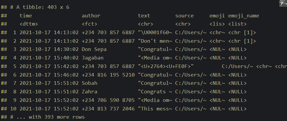
Image by Author

I lost some messages, the messages are actually more than this. We have just 403 messages here.

Let’s see the number of messages sent on a daily basis.

chat %>% 
mutate(day = lubridate::date(time)) %>%
count(day) %>%
ggplot(aes(x = day, y = n)) +
geom_bar(stat = "identity") +
ylab("") +
xlab("") +
ggtitle("Messages per day")
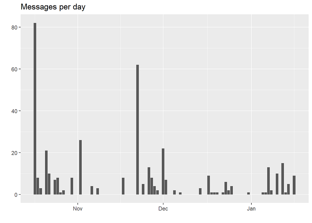
Recently the group hasn’t been active as before.

The number of messages sent daily has dropped.

As of December, the maximum number of messages sent hasn’t been more than 20 messages per day. Seems everybody is busy with life (lol!). Let’s see the active members.

chat %>% 
mutate(day = lubridate::date(time)) %>%
count(author) %>%
arrange(desc(n)) %>%
head() %>%
ggplot(aes(x = reorder(author, n), y = n, fill = author)) + geom_bar(stat = "identity") +
ylab("") +
xlab("") +
coord_flip() +
ggtitle("Number of messages")
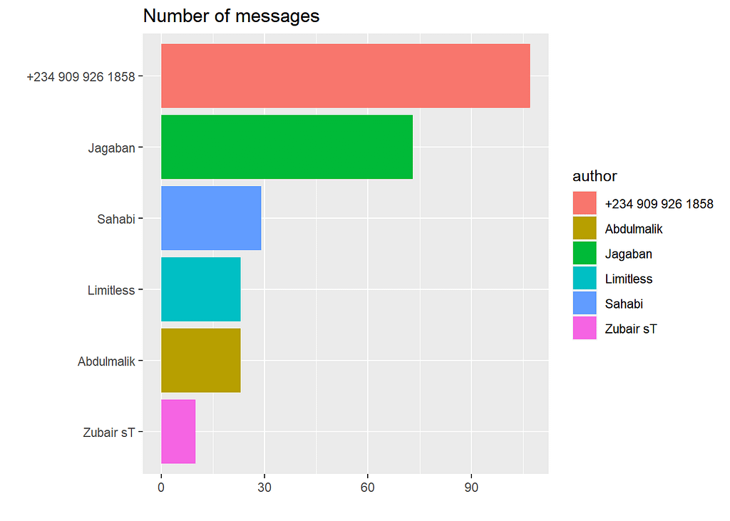
More than 90 messages have been sent by an unknown number.

Jagaban is the group admin, as expected of him, he is regularly active.

Let’s get to the fun part, lets see the most often used emojis in the group.

library("ggimage") emoji_data <- 
rwhatsapp::emojis %>% # data built into package mutate(hex_runes1 = gsub("\\s.*", "", hex_runes)) %>% # ignore combined emojis mutate(emoji_url = paste0("https://abs.twimg.com/emoji/v2/72x72/", tolower(hex_runes1), ".png"))
chat %>% 
unnest(emoji) %>%
count(author, emoji, sort = TRUE) %>%
arrange(desc(n)) %>% head(10) %>%
group_by(author) %>%
left_join(emoji_data, by = "emoji") %>%
ggplot(aes(x = reorder(emoji, n), y = n, fill = author)) + geom_col(show.legend = FALSE) +
ylab("") + xlab("") +
coord_flip() +
geom_image(aes(y = n + 20, image = emoji_url)) +
facet_wrap(~author, ncol = 2, scales = "free_y") +
ggtitle("Most often used emojis") +
theme(axis.text.y = element_blank(), axis.ticks.y = element_blank())
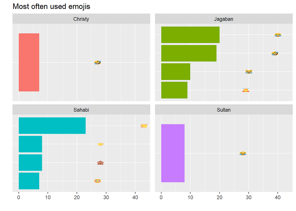
Looks like the most popular emoji is the face with tears of joy. The group admin Jagaban is also the member that sends the most emoji. Let's compare favorite words.

library(tidytext) 
chat %>%
unnest_tokens(input = text, output = word) %>%
count(author, word, sort = TRUE) %>%
head(80) %>%
group_by(author) %>%
top_n(n = 6, n) %>%
ggplot(aes(x = reorder_within(word, n, author), y = n, fill = author)) +
geom_col(show.legend = FALSE) +
ylab("") +
xlab("") +
coord_flip() +
facet_wrap(~author, ncol = 2, scales = "free_y") + scale_x_reordered() +
ggtitle("Most often used words")
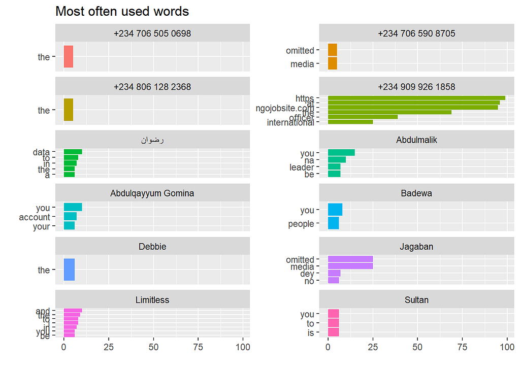
First of all, we have to do is remove the words “media” and “omitted”, these are placeholders Whats app puts into the log file instead of pictures or video.

There are other words that don’t look particularly useful either, these words are called stopwords: words that don’t carry substantial meaning e.g, and, or, and so on. There are some pidgin words also that need to be removed such as dey, na, and so on.

Pidgin words are slang used in Nigeria, if you have been to Nigeria before you will know what I am talking about.

library("stopwords") 
to_remove <- c(stopwords(language = "en"), "media","omitted","na","2","s","u","ahni","irc","dey","3","au","mak","u","don","naa","4","6","una","b","oo","2021","go","sir") chat %>% unnest_tokens(input = text, output = word) %>% 
filter(!word %in% to_remove) %>%
count(author, word, sort = TRUE) %>%
head(90) %>% group_by(author) %>%
top_n(n = 6, n) %>%
ggplot(aes(x = reorder_within(word, n, author), y = n, fill = author)) +
geom_col(show.legend = FALSE) + ylab("") +
xlab("") +
coord_flip() +
facet_wrap(~author, ncol = 2, scales = "free_y") + scale_x_reordered() + ggtitle("Most often used words")
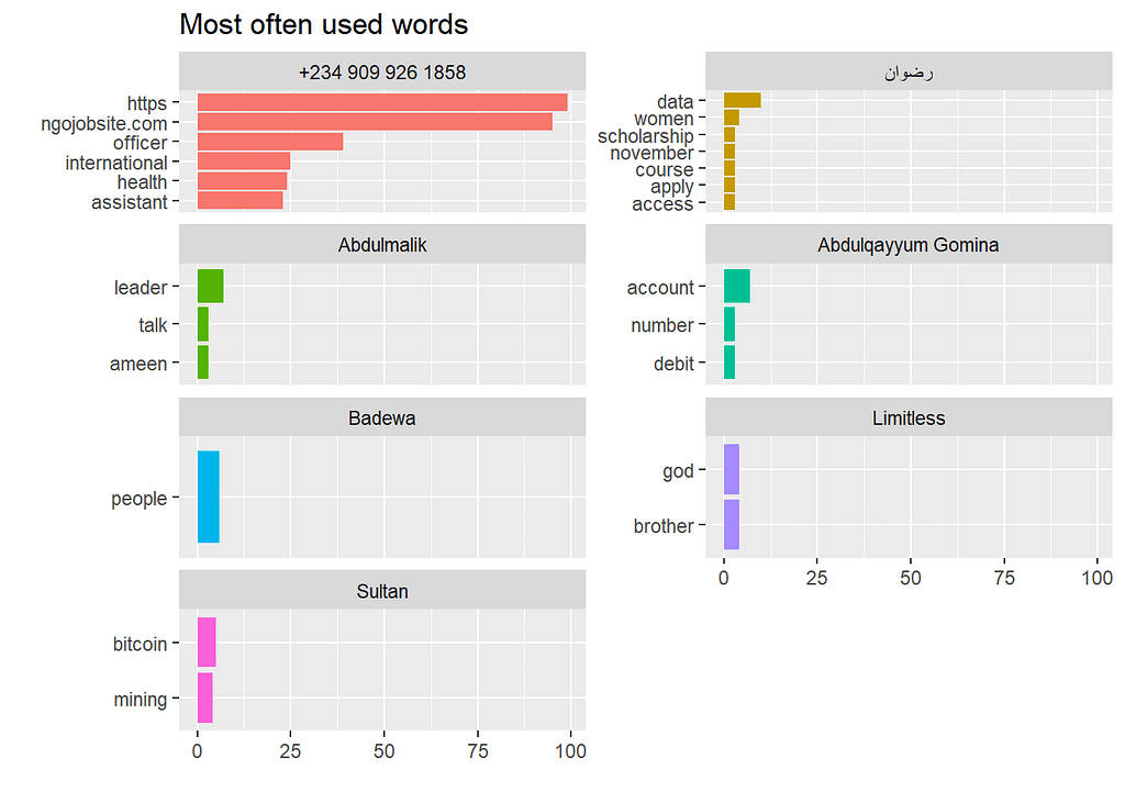
The unknown number sends more links which are mostly job links from the link name ngojobsite.com in the group chat.

Another text mining technique we can do is to calculate lexical diversity. This allows us to see how many unique words are used by an author.

chat %>% 
unnest_tokens(input = text, output = word) %>%
filter(!word %in% to_remove) %>%
count(author, word, sort = TRUE) %>%
group_by(author) %>%
summarise(lex_diversity = n_distinct(word)) %>% arrange(desc(lex_diversity)) %>%
head(10) %>%
ggplot(aes(x = reorder(author, lex_diversity), y = lex_diversity, fill = author)) +
geom_col(show.legend = FALSE) +
scale_y_continuous(expand = (mult = c(0, 0, 0, 500))) + geom_text(aes(label = scales::comma(lex_diversity)), hjust = -0.1) + ylab("unique words") +
xlab("") +
ggtitle("Lexical Diversity") +
coord_flip()
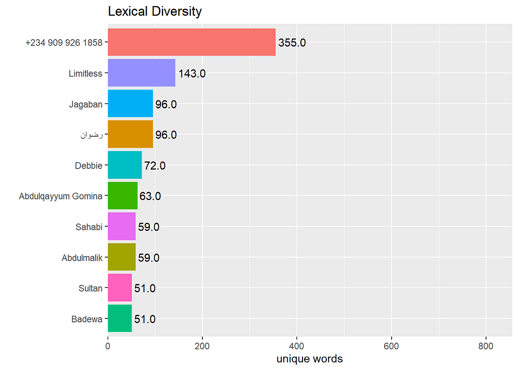
From previous plots, we know that the unknown number mostly shares website links.

Let’s see what the unique words used by Limitless who is the second on the list.

o_words <- chat %>% 
unnest_tokens(input = text, output = word) %>%
filter(author != "Limitless") %>%
count(word, sort = TRUE) chat %>%
unnest_tokens(input = text, output = word) %>%
filter(author == "Limitless") %>%
count(word, sort = TRUE) %>%
filter(!word %in% o_words$word) %>% # only select words nobody else uses top_n(n = 6, n) %>%
ggplot(aes(x = reorder(word, n), y = n, fill = word)) + geom_col(show.legend = FALSE) +
ylab("") +
xlab("") +
coord_flip() +
ggtitle("Unique words of Limitless")
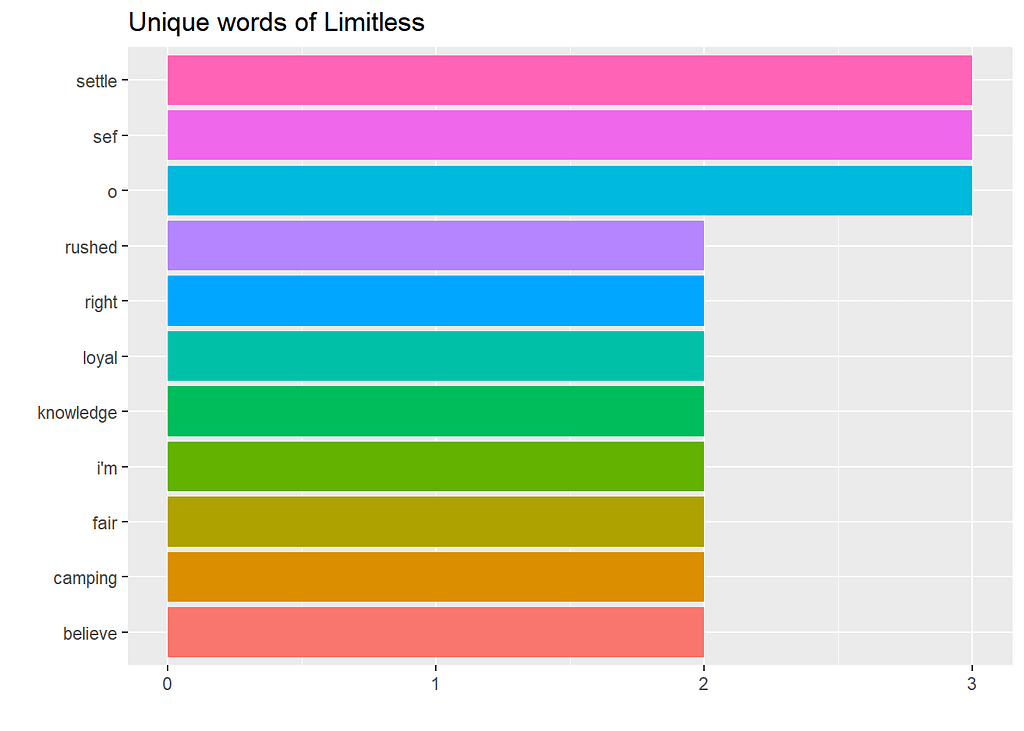
Seeing from the above, these are words that are unique to Limitless.

You can perform a similar analysis on your data and even do better.

Originally published at https://www.adejumoridwan.com on January 16, 2022.

Level Up Coding

Thanks for being a part of our community! Before you go:

🚀👉 Join the Level Up talent collective and find an amazing job


How To Analyze Your WhatsApp Data With R Programming. was originally published in Level Up Coding on Medium, where people are continuing the conversation by highlighting and responding to this story.


This content originally appeared on Level Up Coding - Medium and was authored by Adejumo Ridwan Suleiman


Print Share Comment Cite Upload Translate Updates
APA

Adejumo Ridwan Suleiman | Sciencx (2022-11-28T12:46:49+00:00) How To Analyze Your WhatsApp Data With R Programming.. Retrieved from https://www.scien.cx/2022/11/28/how-to-analyze-your-whatsapp-data-with-r-programming/

MLA
" » How To Analyze Your WhatsApp Data With R Programming.." Adejumo Ridwan Suleiman | Sciencx - Monday November 28, 2022, https://www.scien.cx/2022/11/28/how-to-analyze-your-whatsapp-data-with-r-programming/
HARVARD
Adejumo Ridwan Suleiman | Sciencx Monday November 28, 2022 » How To Analyze Your WhatsApp Data With R Programming.., viewed ,<https://www.scien.cx/2022/11/28/how-to-analyze-your-whatsapp-data-with-r-programming/>
VANCOUVER
Adejumo Ridwan Suleiman | Sciencx - » How To Analyze Your WhatsApp Data With R Programming.. [Internet]. [Accessed ]. Available from: https://www.scien.cx/2022/11/28/how-to-analyze-your-whatsapp-data-with-r-programming/
CHICAGO
" » How To Analyze Your WhatsApp Data With R Programming.." Adejumo Ridwan Suleiman | Sciencx - Accessed . https://www.scien.cx/2022/11/28/how-to-analyze-your-whatsapp-data-with-r-programming/
IEEE
" » How To Analyze Your WhatsApp Data With R Programming.." Adejumo Ridwan Suleiman | Sciencx [Online]. Available: https://www.scien.cx/2022/11/28/how-to-analyze-your-whatsapp-data-with-r-programming/. [Accessed: ]
rf:citation
» How To Analyze Your WhatsApp Data With R Programming. | Adejumo Ridwan Suleiman | Sciencx | https://www.scien.cx/2022/11/28/how-to-analyze-your-whatsapp-data-with-r-programming/ |

Please log in to upload a file.


There are no updates yet.
Click the Upload button above to add an update.

You must be logged in to translate posts. Please log in or register.