Few lines of Python code can generate datasets comparison report. Here is HOW.

A few lines of Python code can generate comparison report for two datasets

Using Pandas Profiling to compare and analyze two datasets

Photo by Isaac Smith on Unsplash

Data visualization is the fundamental of Exploratory Data Analysis (EDA). When faced with a new, unknown dataset, visual inspection allows us to discover useful information, draw some patterns about the data, and diagnose problems that we may need to solve. In this regard, Pandas Profiling has been an indispensable “Swiss knife” in every data scientist’s toolbox, which can help us quickly generate data summary reports, including data overview, variable attributes, distributions, repeated values and other indicators. Pandas Profiling is able to present these information in visualizations so that we can better understand the dataset. But what if we were able to compare two datasets, is there an easiest way to do it?

In this article, I will describe how to use Pandas Profiling’s comparative reporting capabilities to enhance the your exploratory data analysis (EDA) process. I will introduce how to compare two different datasets by Pandas Profiling, which can help us compare and analyze data faster, and find out distribution differences for further data exploration.

Preparation

The dataset I use for demonstration is based on “HCC (Hepatocellular carcinoma) dataset” downloaded from Kaggle: https://www.kaggle.com/datasets/mrsantos/hcc-dataset/versions/5. We will use the file “hcc-data-complete-balanced.csv”. As we are going to compare the datasets one after manual distortion and the other after correction in order to see the comparison from report, firstly we intend to make a little changes on original HCC dataset. We will create three typical data issues which happened normally in our datasets of daily research, but before that, let’s reduce column number from the dataset for better visual explanation:

Three data issues created intentionally as below:

a) Create new column with constant value — column “O2” with all the value being 999.
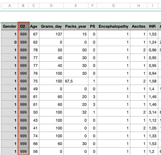
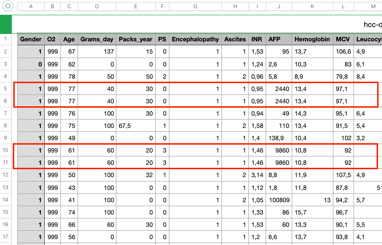
b) Duplicate rows — two rows copied from their above one.
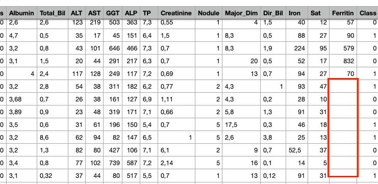
c) Delete some data in column “Ferritin”
Then, let’s do some quick data exploration on this new dataset by using Pandas Profiling.

Original reporting

Firstly, we need to download and install pandas-profiling package via pip.

$ pip install pandas-profilin==3.5.0

The code for Profile Report generation is simple:

import pandas as pd
from pandas_profiling import ProfileReport

df = pd.read_csv("hcc-data-complete-balanced.csv")

original_report = ProfileReport(df, title='Original Data')
original_report.to_file("original_report.html")

From the “Alerts” tab of the report html page “original_report.html” in notebook working directory, we observed a couple of potential risks we expected from Pandas Profiling analysis:
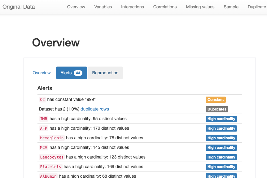
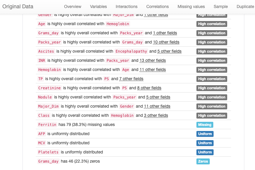
There are several categories of alerts listed in the report:

  • Constant: ‘O2’ is a constant factor as all of the values are 999
  • Duplicates: There are two duplicated rows
  • High cardinality: These fields have very distinct values in its column
  • High correlation: These fields have strong relevance with each other
  • Missing: “Ferritin” has missing values

Data Handling

Let’s write a couple of lines of code to fix these issues we care about:

Remove the duplicates

In the dataset, some features are very specific and refer to individual biometric values, such as hemoglobin, MCV, albumin, etc. Therefore, it is impossible to have multiple patients reporting the same exact values for all fields. That’s why we can simply remove these duplicates:

df_transformed = df.copy()
df_transformed = df_transformed.drop_duplicates()

Remove the useless fields

During data analysis, some features may not have much value, such as the O2 constant value. Removing these fields will help in the development of the model.

df_transformed = df_transformed.drop(columns='O2')

Compensate the missing data

Data imputation is a method used to compensate missing data. It allows us to impute missing values without removing observation values. Mean imputation (MI), the most common and simplest statistical imputation method, calculates the mean of a feature to fill in missing values. We use MI to handle missing data in our dataset:

from sklearn.impute import SimpleImputer
mean_imputer = SimpleImputer(strategy="mean")
df_transformed['Ferritin'] = mean_imputer.fit_transform(df_transformed['Ferritin'].values.reshape(-1,1))

Comparative Analysis

Now we have two datasets, one has some defects and the other fixed them. We are going to make use of them to demonstrate the advanced comparison feature of Pandas Profiling. The code is much simple with Python to generate comparison report:

transformed_report = ProfileReport(df_transformed, title="Transformed Data")
comparison_report = original_report.compare(transformed_report)
comparison_report.to_file("original_vs_transformed.html")

Find the report “original_vs_transformed.html” in your notebook working directory, open it in the browser:
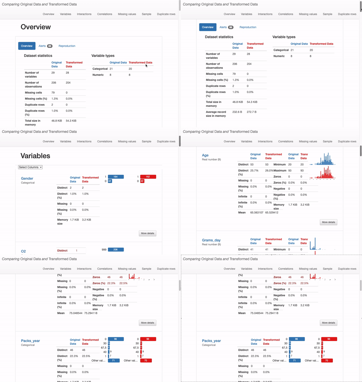
What can we immediately learn from the dataset overview?

  • The transformed dataset contains fewer features (“O2” has been removed)
  • 204 observations (versus original 206 including duplicates)
  • There are no missing values (in contrast to the 79 missing observations in the original dataset).

How does this shift affect our data quality? Are these designs good or bad? In fact, we found that there is no special impact on deleting duplicate and constant records, there are some actual changes in missing data from data distribution issue, as shown in the following figure:
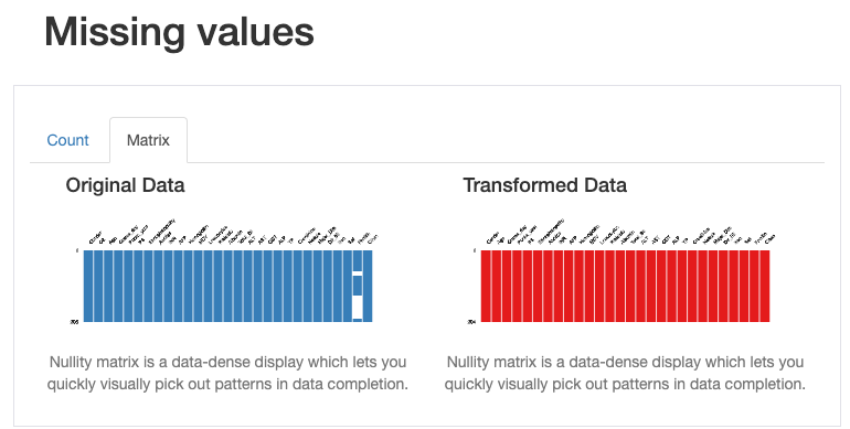
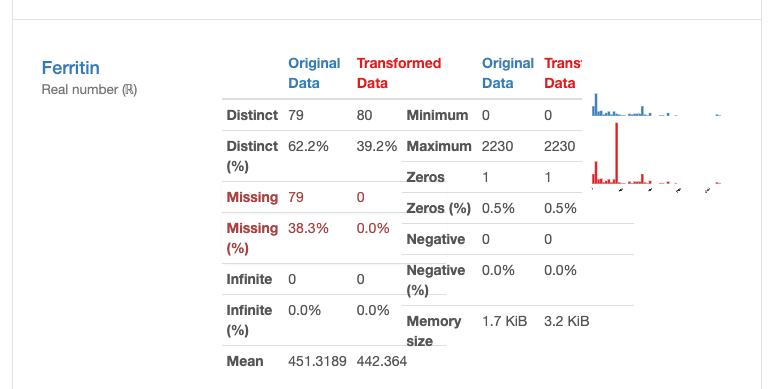
From the above illustration, it can be seen that some information, such as for the “ferritin” field, the mean estimate of the imputation data causes the distribution of the original data to be distorted. This can be problematic, and we should avoid using mean estimates to replace missing values. In this case, other methods should be used to deal with missing values, such as removing missing values or using other statistical methods to impute missing values.

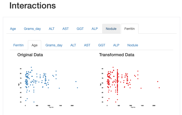
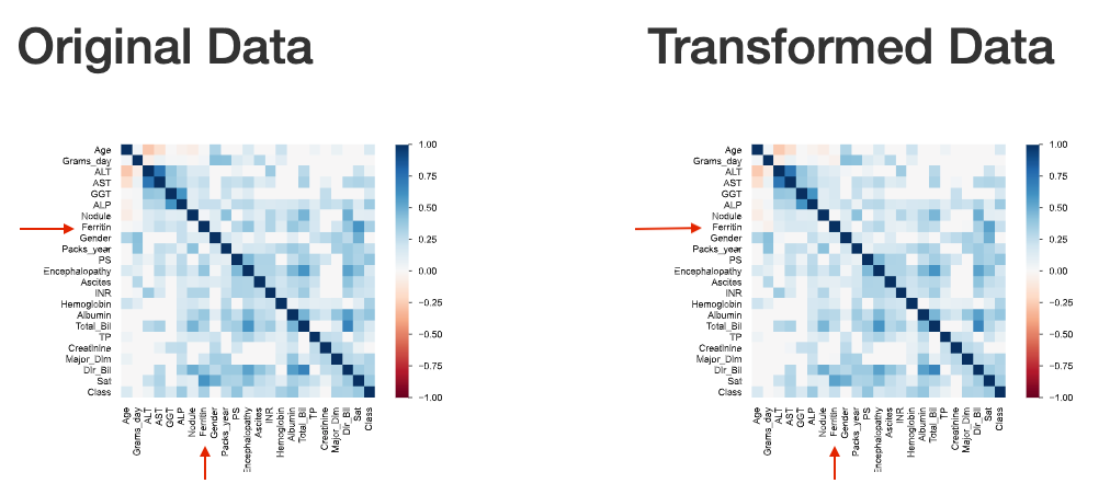
This can also be observed through the visualization of interactions and correlations, where inconsistent interaction patterns and higher correlation values exists between ‘ferritin’ and other features.
Estimated values are shown on the vertical line corresponding to the mean imputation interactive between ferritin and age:
The ferritin correlation with other fields’ values seem to decrease after data imputation (becomes higher color temperature in below figure).
Conclusion

In this article, I explained how the Pandas Profiling tool compares and analyzes different datasets. We used the data before and after correction to make a simple demonstration. In fact, this method can also be used in the comparison between training set and test set to find problems such as data shifting, etc.

Level Up Coding

Thanks for being a part of our community! Before you go:

🚀👉 Join the Level Up talent collective and find an amazing job


Few lines of Python code can generate datasets comparison report. Here is HOW. was originally published in Level Up Coding on Medium, where people are continuing the conversation by highlighting and responding to this story.


This content originally appeared on Level Up Coding - Medium and was authored by Yeyu Huang


Print Share Comment Cite Upload Translate Updates
APA

Yeyu Huang | Sciencx (2023-01-17T12:19:49+00:00) Few lines of Python code can generate datasets comparison report. Here is HOW.. Retrieved from https://www.scien.cx/2023/01/17/few-lines-of-python-code-can-generate-datasets-comparison-report-here-is-how/

MLA
" » Few lines of Python code can generate datasets comparison report. Here is HOW.." Yeyu Huang | Sciencx - Tuesday January 17, 2023, https://www.scien.cx/2023/01/17/few-lines-of-python-code-can-generate-datasets-comparison-report-here-is-how/
HARVARD
Yeyu Huang | Sciencx Tuesday January 17, 2023 » Few lines of Python code can generate datasets comparison report. Here is HOW.., viewed ,<https://www.scien.cx/2023/01/17/few-lines-of-python-code-can-generate-datasets-comparison-report-here-is-how/>
VANCOUVER
Yeyu Huang | Sciencx - » Few lines of Python code can generate datasets comparison report. Here is HOW.. [Internet]. [Accessed ]. Available from: https://www.scien.cx/2023/01/17/few-lines-of-python-code-can-generate-datasets-comparison-report-here-is-how/
CHICAGO
" » Few lines of Python code can generate datasets comparison report. Here is HOW.." Yeyu Huang | Sciencx - Accessed . https://www.scien.cx/2023/01/17/few-lines-of-python-code-can-generate-datasets-comparison-report-here-is-how/
IEEE
" » Few lines of Python code can generate datasets comparison report. Here is HOW.." Yeyu Huang | Sciencx [Online]. Available: https://www.scien.cx/2023/01/17/few-lines-of-python-code-can-generate-datasets-comparison-report-here-is-how/. [Accessed: ]
rf:citation
» Few lines of Python code can generate datasets comparison report. Here is HOW. | Yeyu Huang | Sciencx | https://www.scien.cx/2023/01/17/few-lines-of-python-code-can-generate-datasets-comparison-report-here-is-how/ |

Please log in to upload a file.


There are no updates yet.
Click the Upload button above to add an update.

You must be logged in to translate posts. Please log in or register.