
This content originally appeared on Level Up Coding - Medium and was authored by Aydin Schwartz

Data scientists and engineers are not always lucky enough to be working with nicely-labeled datasets. If we’re given a bunch of unlabeled data, how do we start to make sense of it? The answer is clustering.
The aim of clustering is to identify areas in data where observations naturally group together. By identifying patterns and similarities within the data, clustering algorithms can help us gain insights into its underlying structure. This simple idea has applications in many domains, from fraud detection to image compression.
There are many different types of clustering algorithms out there, each with its own strengths and limitations. In this article I want to explain and create visual intuition for two of the most popular: k-means clustering and DBSCAN.
K-Means Clustering
K-means is one of the most well-known and widely used clustering algorithms. The “k” in its name refers to the amount of clusters that must be found in the data. This is a parameter of the model that the user must decide on, either through experimentation or domain knowledge.
Initially, the algorithm generates k “centroids” randomly scattered around the data. These are the points that will serve as the centers of our clusters. K-means then assigns each data point to its nearest centroid. The centroids are then updated, with their new values being the mean of the data points that have been assigned to them.
At this point, some data points that started closest to one centroid will be closer to a different centroid. So we run the whole process again to create the next iteration of clusters. The algorithm continues until either no data points change clusters after an update, or it reaches predefined number of iterations. The entire k-means algorithm can be defined in a few simple steps:
1. Choose the number of clusters k
2. Initialize k centroids randomly
3. Repeat until convergence:
   a. Assign each data point to the nearest centroid
   b. Update each centroid to the mean of the assigned data points
In the real world, we’re usually running k-means on many-dimensional data that can’t be easily visualized. However, to better explain the nature of the algorithm, we can run k-means on two-dimensional data with clear and recognizable clusters.
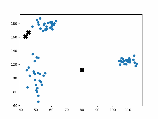
Initially, the centroids are placed randomly throughout the feature space. As we iterate through the steps of the algorithm, the centroids separate quickly and easily into their own clusters. In the example above, the orange cluster actually stopped changing after the very first iteration. Unfortunately, this idyllic scenario does doesn’t always happen. This version of k-means clustering does not have a deterministic outcome. Its performance depends heavily on the random placement of the initial centroids. There are many possible stable clusterings where the placement of the centroids is completely incorrect.
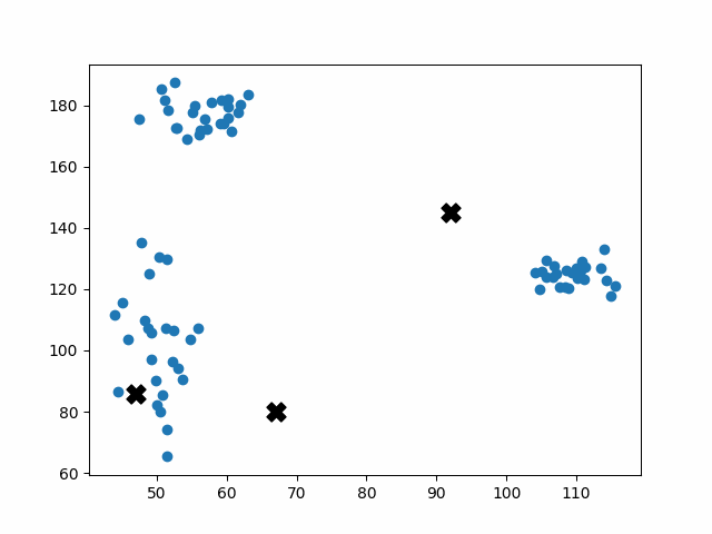
This unfortunate condition can be mitigated by choosing better starting centroids.
K-Means++
The k-means++ method is a modification to the original k-means algorithm that significantly improves the runtime of the algorithm and the quality of its clusterings. Surprisingly, it leaves the core of the original algorithm unchanged. The only difference is in how it selects the first centroid positions.
Instead of generating centroids anywhere in the dimension of the data, each centroid is initialized on top of an existing data point. The first centroid is chosen randomly, and each subsequent centroid is chosen to maximize the minimum distance from the centroids that have already been created. This simple change to the initialization of the k-means algorithm creates clusters that are more balanced and stable. Note that there are multiple different implementations of kmeans++, but they all share the same goal of selecting better initial cluster centers. This procedure can be summarized in the following way:
1. Pick first centroid randomly from the data points
2. For each remaining centroid:
   a. Compute the closest centroid to each data point
   b. Choose the data point that is furthest away from its closet centroid
      as the next centroid
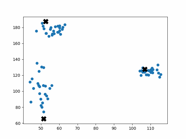
K-means++ tends to enjoy faster convergence to a stable clustering than random initialization does, and the graphics above provide some insight into why this is the case. Since centroids are initialized far away from each other, they don’t fight as much over data. Points are less likely to jump back and forth between different clusters. Also, each centroid is more likely to be initialized by itself inside of a true cluster. By contrast, random initialization can create multiple centroids in the middle of a cluster, leading them to divide the cluster arbitrarily.
Sadly, k-means++ doesn’t solve all of our problems. An insurmountable limitation of the k-means algorithm is that it operates under the assumption that the clusters are distributed around a central point (globular). This idea is fundamental to the operation of k-means, and we cannot optimize our way out of it. This means that k-means will perform poorly on non-globular data, such as elongated or irregularly shaped clusters.
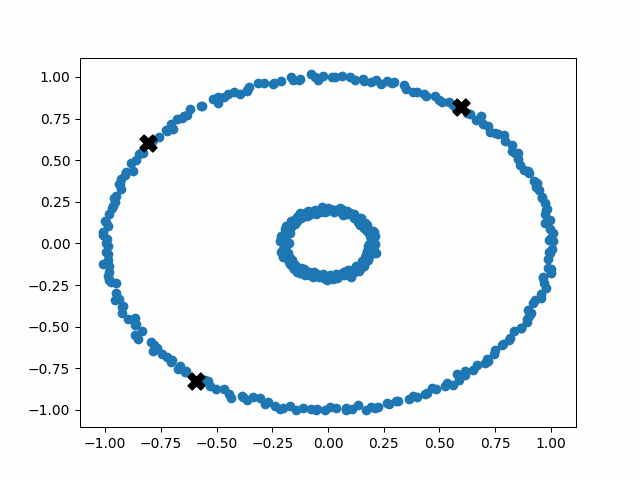
In order to tackle this new problem, we need an algorithm that holds fewer assumptions about the general distribution of a cluster.
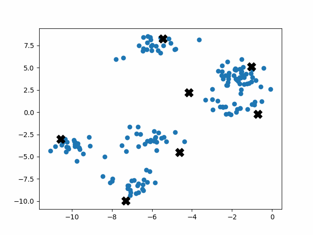
DBSCAN
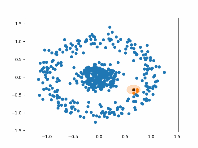
DBSCAN stands for Density-Based Spatial Clustering of Applications with Noise. What a mouthful. Like k-means, however, the fundamental idea of DBSCAN is simple: data points packed tightly next to other data points likely share the same cluster.
DBSCAN does not require us to specify the number of clusters beforehand like k-means does. Instead, it requires two parameters typically denoted as minPoints and eps (short for epsilon). They are defined as follows:
- minPoints: The minimum number of neighbors a point needs in order to be considered a “core point” of a cluster.
- eps: The length of a radius that will be used as the search boundary for the nearest neighbors of a given point.
DBSCAN also identifies three different types of points:
- Core points: points that have at least minPoints number of other points within a distance of eps. They form the main body of a cluster.
- Non-core points: points that have less than minPoints number of points within a distance of eps, but are within the radius of a core point. They are still part of the cluster.
- Noise points: points that do not have any core points within their radius. They are not part of any cluster, regardless of how many non-core points they have as neighbors.
The algorithm operates in the following way:
1. Select a random, unvisited point from the dataset.
2. Find all the neighboring points within a distance of eps from the
   selected point.
3. If the number of neighboring points >= minPoints, label the point as a
   core point and marked it as visited. Assign it a new cluster label.
   a. Check neighbors to see if are core points. If they are not,
      mark them as non-core points and do not check their neighbors.
      If they are, expand the cluster by checking their neighbors. Either
      way mark them as visited and add them to the cluster.
   b. Continue until you run out of unvisited neighbors.
4. Select the next unvisited point from the dataset and repeat until all
   points are visited.
Basically, a cluster will keep expanding as long as it runs into core points. Non-core points are part of the cluster but do not help it expand, and tend to form the border of a cluster. Noise points are just points that were so far from the core of any cluster that they were ignored.
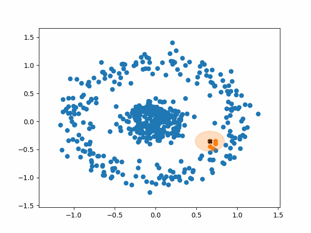
Using this density-based criteria for cluster creation allows DBSCAN to successfully handle a huge variety of data. Additionally, DBSCAN is robust to outliers. K-means must put every point in the data into a cluster, whereas DBSCAN will simply ignore points that it classifies as noise.
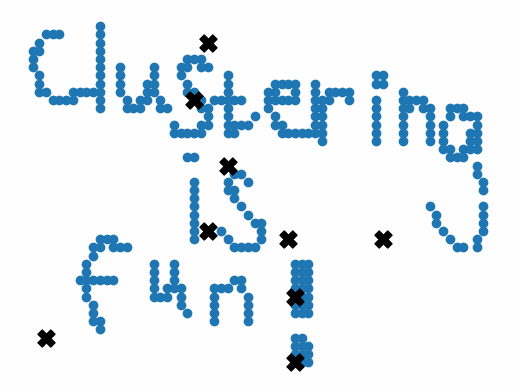
Still, DBSCAN has its issues. One such limitation is that it requires careful parameter selection. Choosing the right values for eps and minPoints can be challenging, and poor parameter selection can lead to useless clustering results.
Bonus: Image Compression
These 2D visualizations of clustering are fun, but what are they actually useful for? One really interesting application is image compression. Using clustering algorithms, we can dramatically reduce the amount of colors and data in an image without significantly affecting its quality.
First, we take an image and treat each pixel as a data point with its red, green, and blue (RGB) values in 3D space. The k-means algorithm can then be applied to classify these data points into k clusters, where k is the desired number of colors in the compressed image. The centroids of the k clusters represent the k colors to be used in the compressed image. Each pixel in the original image is then replaced by the centroid of the cluster to which it belongs.


The result is a compressed image with only k colors, which can significantly reduce the file size of the image. If k is large enough, the image can be recreated without any noticeable loss in visual quality. Most original photos contain a limited number of dominant colors, and k-means clustering can effectively capture these colors, making the change imperceptible to the human eye.
Final Thoughts
This article only scratched the surface in terms of existing clustering algorithms and applications. I hope that you were able to gain some intuition about the nature of k-means and DBSCAN from this article. For further reading, I highly recommend this article by David Sheehan. It explains a bunch of clustering algorithms using some truly fantastic visuals.
Thanks for reading!
Level Up Coding
Thanks for being a part of our community! Before you go:
- 👏 Clap for the story and follow the author 👉
- 📰 View more content in the Level Up Coding publication
- 💰 Free coding interview course ⇒ View Course
- 🔔 Follow us: Twitter | LinkedIn | Newsletter
🚀👉 Join the Level Up talent collective and find an amazing job
Visualizing Clustering Algorithms: K-Means and DBSCAN was originally published in Level Up Coding on Medium, where people are continuing the conversation by highlighting and responding to this story.
This content originally appeared on Level Up Coding - Medium and was authored by Aydin Schwartz
Aydin Schwartz | Sciencx (2023-03-23T23:22:33+00:00) Visualizing Clustering Algorithms: K-Means and DBSCAN. Retrieved from https://www.scien.cx/2023/03/23/visualizing-clustering-algorithms-k-means-and-dbscan/
Please log in to upload a file.
There are no updates yet.
Click the Upload button above to add an update.