
This content originally appeared on Level Up Coding - Medium and was authored by Guglielmo Cerri

Introduction
Machine learning is a powerful field that enables computers to learn from data and make predictions or decisions without being explicitly programmed. This article provide a beginner-friendly introduction to machine learning concepts and demonstrate how to implement them using Python. We’ll cover essential topics such as classification, regression, clustering and image recognition.
We will utilize the scikit-learn library in Python, which provides a wide range of machine learning algorithms and tools and the TensorFlow library which provides a comprehensive set of tools for building and training deep learning models.
1. Classification
Classification is a supervised learning technique that involves the use of labeled data to train a model to make predictions on unseen or future instances. In supervised learning, the dataset consists of input features along with their corresponding class or label. The classification algorithm analyzes the relationship between the input features and the known classes to build a model that can generalize and make accurate predictions on new, unseen data.
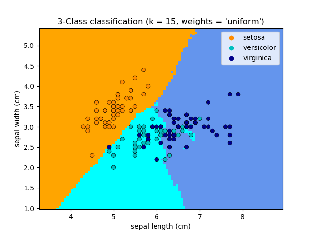
Our goal is to build a classification model that can predict the species of an Iris flower (discrete value) based on its measurements.

First, we will load the Iris dataset, which is conveniently available in scikit-learn. The dataset is split into two arrays: one containing the feature values (X) and the other containing the corresponding target labels (y).
The dataset consists of measurements of four features (sepal length, sepal width, petal length, and petal width) for three different species of Iris flowers (setosa, versicolor, and virginica).
Next, we will split the dataset into training and testing sets using the train_test_split function from scikit-learn. This step ensures that we have separate data for training and evaluating our classification model.
To perform the classification, we will use the k-nearest neighbors (KNN) classifier. KNN is a simple yet effective algorithm that classifies new data points based on the majority vote of their k nearest neighbors in the training set. We will initialize the KNN classifier, fit it to the training data, and make predictions on the testing data.
To evaluate the quality of the model’s predictions we use the balanced accuracy score, which is a metric that takes into account the imbalance in the number of samples across different classes. It provides a fair assessment of the classifier’s performance in scenarios where the classes are not equally represented.
By calculating the balanced accuracy score, we can assess how well our classification model performs on the testing set. The higher the score, the better the model’s ability to correctly classify the Iris flowers.
Once we have chosen the model, we can also make predictions on new, unseen Iris flowers by providing their feature values to the classifier’s predict method. The model will assign a predicted species label to each new data point based on its measurements.
Code:
from sklearn import datasets
from sklearn.model_selection import train_test_split
from sklearn.neighbors import KNeighborsClassifier
from sklearn.metrics import balanced_accuracy_score

# Load the Iris dataset
iris = datasets.load_iris()
X = iris.data
y = iris.target

# Split the data into training and testing sets
X_train, X_test, y_train, y_test = train_test_split(X, y, test_size=0.2)

# Train a k-nearest neighbors classifier
clf = KNeighborsClassifier()
clf.fit(X_train, y_train)

# Make predictions on the testing set
y_pred = clf.predict(X_test)

# Evaluate the model using balanced accuracy score
accuracy = balanced_accuracy_score(y_test, y_pred)
print("Balanced Accuracy: ", accuracy)

# Make predictions on new data
new_data = [[5.1, 3.5, 1.4, 0.2], [6.7, 3.0, 5.2, 2.3]]  # Example new data
predicted_labels = clf.predict(new_data)
2. Regression
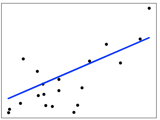
Regression is a statistical modeling technique used to predict continuous numerical values based on input features. Unlike classification, which predicts discrete class labels, regression aims to estimate a continuous outcome variable or target variable.
In this example, we will explore regression using the California Housing dataset. It contains information about various housing features in different districts of California, such as population, median income, and median house prices.
Our goal is to build a regression model that can predict the median house prices (continuous value) based on the given features.
To start, we load the dataset. As for the previous one, it consists of a feature matrix (X) containing the housing features and a corresponding target vector (y) indicating the median house prices.
Next, we will preprocess the data by scaling the features and splitting it into training and testing sets. Scaling is important to ensure that all features contribute equally to the regression model.
We will then select a regression algorithm, such as linear regression, and train the model using the training data. Once the model is trained, we will evaluate its performance using mean squared error (MSE) metric, that measures the average of the squared differences between the predicted values and the actual values of a variable.
Code:
from sklearn.datasets import fetch_california_housing
from sklearn.model_selection import train_test_split
from sklearn.linear_model import LinearRegression
from sklearn.metrics import mean_squared_error

# Load the California Housing dataset
california_housing = fetch_california_housing()
X = california_housing.data
y = california_housing.target

# Preprocess the data
# (Scaling, splitting into training and testing sets)

X_train, X_test, y_train, y_test = train_test_split(X, y, test_size=0.2, random_state=42)

# Build and train the regression model
model = LinearRegression()
model.fit(X_train, y_train)

# Make predictions on the testing set
y_pred = model.predict(X_test)

# Evaluate the model
mse = mean_squared_error(y_test, y_pred)
print("Mean Squared Error:", mse)
3. Clustering
Clustering is an unsupervised learning technique that helps identify inherent patterns and structures within the data. It is particularly useful when the true labels or categories are not known in advance. By grouping similar data points together, clustering enables us to gain insights into the underlying structure of the data and discover meaningful relationships.
In this example, we use the K-means algorithm to group similar Iris flowers together based on their feature measurements. We will also plot the clusters to visualize the results.
To begin, we will load the Iris dataset, and divided it into X and y values.
Next, we will apply the K-means clustering algorithm to the dataset that aims to partition the data into K distinct clusters, where each data point belongs to the cluster with the nearest mean (centroid). We will initialize the K-means model with the desired number of clusters, fit it to the data, and obtain the cluster labels for each data point.
To visualize the clusters, we use a scatter plot. Each point represents an Iris flower sample, and the color of the point indicates its assigned cluster. Additionally, we plotted the centroids of the clusters as red stars.
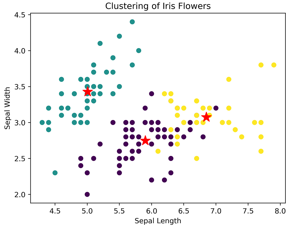
The plot helps us understand how the K-means algorithm grouped the Iris flowers based on their measurements. It provides insights into the distinct clusters and their separation in the feature space.
Feel free to modify the number of clusters (n_clusters) and explore different visualizations to gain a deeper understanding of clustering and its application to real-world datasets.
Code:
import matplotlib.pyplot as plt
from sklearn.cluster import KMeans
from sklearn.datasets import load_iris

# Load the Iris flower dataset
iris = load_iris()
X = iris.data

# Apply the K-means algorithm
kmeans = KMeans(n_clusters=3, random_state=42, n_init=10)
clusters = kmeans.fit_predict(X)

# Plot the clusters
plt.scatter(X[:, 0], X[:, 1], c=clusters)
plt.scatter(kmeans.cluster_centers_[:, 0], kmeans.cluster_centers_[:, 1], marker='*', color='red', s=200)
plt.xlabel('Sepal Length')
plt.ylabel('Sepal Width')
plt.title('Clustering of Iris Flowers')
plt.show()
4. Image Recognition
Image recognition, also known as computer vision, is a field of study in which machines are trained to analyze and interpret images or visual data. It involves developing algorithms and models that can understand the content, objects, and patterns present in images and make predictions or classifications based on them. This can involve tasks such as object detection, object localization, image classification, and image segmentation.
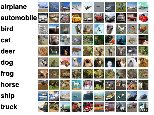
To complete this tutorial, we will dive into the field of image classification using the CIFAR-10 dataset. It is a popular benchmark in computer vision, consisting of 60,000 color images (32x32 pixels) across ten different classes, such as airplanes, cars, cats, and dogs.
Our goal is to build a neural network that can accurately classify images into their respective categories.
After loading the dataset, which can be easily accessed through TensorFlow’s built-in datasets module, it is splitted into training and testing sets, with images represented as NumPy arrays and corresponding labels indicating the class of each image.
Next, we will preprocess the images by normalizing their pixel values and transforming the labels into one-hot encoded vectors, where we represent each class as a binary vector. This step ensures that the input data is in a suitable format for training a deep learning model.
For image recognition, we will utilize a convolutional neural network (CNN), a type of deep learning architecture well-suited for analyzing visual data. We will define a CNN model using TensorFlow’s high-level API, Keras, and configure its layers, including convolutional, pooling and fully connected layers.
import tensorflow as tf
from tensorflow import keras

# Load the CIFAR-10 dataset
cifar10 = keras.datasets.cifar10
(X_train, y_train), (X_test, y_test) = cifar10.load_data()

# Preprocess the data
X_train = X_train / 255.0
X_test = X_test / 255.0

# Convert categorical labels into a one-hot encoded format
y_train = keras.utils.to_categorical(y_train, num_classes=10)
y_test = keras.utils.to_categorical(y_test, num_classes=10)

# Build a convolutional neural network
model = keras.Sequential([
    keras.layers.Conv2D(32, (3, 3), activation='relu', input_shape=(32, 32, 3)),
    keras.layers.MaxPooling2D((2, 2)),
    keras.layers.Conv2D(64, (3, 3), activation='relu'),
    keras.layers.MaxPooling2D((2, 2)),
    keras.layers.Conv2D(64, (3, 3), activation='relu'),
    keras.layers.Flatten(),
    keras.layers.Dense(64, activation='relu'),
    keras.layers.Dense(10, activation='softmax')
])

# Compile and train the model
model.compile(optimizer='adam', loss='categorical_crossentropy', metrics=['accuracy'])
model.fit(X_train, y_train, epochs=10, batch_size=64)

# Evaluate the model
test_loss, test_accuracy = model.evaluate(X_test, y_test)
print("Test Loss:", test_loss)
print("Test Accuracy:", test_accuracy)
In this example, we are using a CNN model to perform image recognition on the dataset. The model consists of multiple convolutional layers to extract meaningful features from the images, followed by fully connected layers to classify the extracted features.
After defining the model architecture, we compile it with an optimizer and a loss function. We then train the model on the training set using the fit function, specifying the number of epochs (iterations) and the batch size.
Finally, we evaluate the trained model on the test set using a metric error (loss) and a percentage of correctly classified images (accuracy).
Conclusion
In this article, we explored key aspects of machine learning in programming, focusing on classification, regression, clustering, and image recognition. Through practical examples using popular datasets, we showcased the application of these concepts in Python.
We built a classification model using the Iris flower dataset and evaluated its performance using the balanced accuracy score. In regression, we predicted housing prices using the California Housing dataset and measured performance with the mean squared error. For clustering, we grouped similar Iris flowers using the K-means algorithm, revealing hidden patterns. Finally, In image recognition, we employed a convolutional neural network to classify images from the CIFAR-10 dataset.
Machine learning empowers programmers to tackle complex tasks and gain insights from data. These examples serve as starting points for further exploration. Remember, learning is a continuous process, and practice will enhance your skills in applying machine learning techniques to real-world problems.
Embrace the opportunities in machine learning, leverage powerful libraries like scikit-learn and TensorFlow, and continue honing your skills. With accessible technology, you can create innovative solutions at the intersection of machine learning and programming.
Happy coding and machine learning!
I hope you enjoyed reading this article and find it useful for your own purposes.
If you liked this post, you can follow me on Medium. Feel free to share any questions or suggestions with me 🚀.
Level Up Coding
Thanks for being a part of our community! Before you go:
- 👏 Clap for the story and follow the author 👉
- 📰 View more content in the Level Up Coding publication
- 💰 Free coding interview course ⇒ View Course
- 🔔 Follow us: Twitter | LinkedIn | Newsletter
🚀👉 Join the Level Up talent collective and find an amazing job
Mastering Machine Learning Fundamentals using Python was originally published in Level Up Coding on Medium, where people are continuing the conversation by highlighting and responding to this story.
This content originally appeared on Level Up Coding - Medium and was authored by Guglielmo Cerri
Guglielmo Cerri | Sciencx (2023-05-18T02:56:31+00:00) Mastering Machine Learning Fundamentals using Python. Retrieved from https://www.scien.cx/2023/05/18/mastering-machine-learning-fundamentals-using-python/
Please log in to upload a file.
There are no updates yet.
Click the Upload button above to add an update.