This content originally appeared on Level Up Coding - Medium and was authored by Melanee Group

Introduction
In this article, we will follow a systematic approach to fine-tune the logistic regression algorithm’s hyperparameters. Our process will consist of the following steps:
1. Manually adjusting each hyperparameter
2. Evaluating the impact of each hyperparameter on the model’s accuracy
3. Identifying optimal values for the hyperparameters
Once we have determined the best hyperparameters, we will compare the performance of various models using these optimal values. Finally, we will provide a comprehensive analysis of the effectiveness of hyperparameter tuning in enhancing the model’s performance.
Before diving into our primary objective, it’s crucial to address some fundamental concepts related to this subject.
Logistic Regression
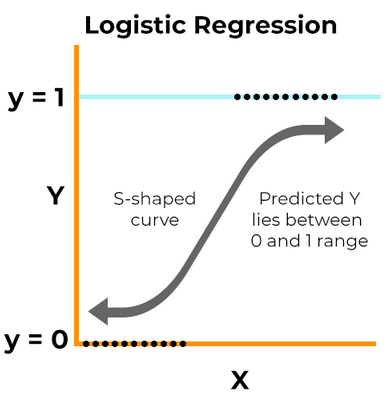
Logistic Regression is a supervised machine learning algorithm and is a linear model for binary classification. In this model, the probabilities that describe the possible outcomes of an experiment are modeled using a logistic function [1].
The logistic function is defined as:
f(x) = L / (1 + e^(-k(x-x0)))
where:
· x: the midpoint values of the sigmoid curve
· L: the maximum value of the curve
· k: the logistic growth rate or the slope of the curve
Here, x represents the input features, and the output is a binary variable (0 or 1). The logistic regression algorithm learns the optimal values of the coefficients from the training data to predict the probability of the binary outcome for new input data. Once the model is trained, it can be used to predict the binary outcome by thresholding the predicted probability [1].
Parameters vs. Hyperparameters
Model parameters and hyperparameters are the two parameter types used in Machine Learning (ML) models. Data estimation or data learning can be used to adjust the model’s parameters. Parameters are values that the model learns from the data, while hyperparameters are values that the user sets to control the behavior of the learning algorithm. Hyperparameters affect how the parameters are learned, and choosing good hyperparameters can be crucial for achieving good performance on a given task. However, the process of optimizing hyperparameters can be complex and time-consuming, especially when dealing with many hyperparameters or multiple optimization objectives. Therefore, it’s important to strike a balance between optimizing hyperparameters and avoiding overfitting the training data [3].
Hyperparameter Tuning
Hyperparameter tuning is a crucial part of the machine learning process as it can significantly affect the performance of the model. By selecting the right hyperparameters, such as learning rate and regularization, among others, a model can achieve optimal performance. However, the process of hyperparameter tuning can be challenging and time-consuming, as there are many hyperparameters to consider, and the search space can be vast. Therefore, it is essential to strike a balance between optimizing the model’s performance and avoiding an endless cycle of trying to optimize [3].
Logistic Regression Hyperparameters
The main hyperparameters we will tune in logistic regression are solver, penalty, max_iter, C (regularization strength), tol, fit_intercept, intercept_scaling, class_weight, random_state, multi_class, verbose, warm_start, and l1_ratio (sklearn documentation) [4].
In the optimization problem, the algorithm to use is called the solver. There are several choices for the solver, including ‘newton-cg’, ‘lbfgs’, ‘liblinear’, ‘sag’, and ‘saga’. The default solver is ‘lbfgs’.
- ‘lbfgs’: This solver performs relatively well compared to other methods and saves a lot of memory. However, it may sometimes have issues with convergence.
- ‘sag’: This solver is faster than other solvers for large datasets, especially when both the number of samples and the number of features are large.
- ‘saga’: This solver is the preferred choice for sparse multinomial logistic regression and is suitable for very large datasets.
- ‘newton-cg’: This solver is computationally expensive due to the Hessian Matrix.
- ‘liblinear’: This solver is recommended for high-dimensional datasets, as it is effective in solving large-scale classification problems [4, 5].
Please note that “sag” and “saga” may only converge quickly when the features have a similar scale. To ensure this, we recommend scaling the data using either StandardScaler or MinMaxScaler from the sklearn.preprocessing module before fitting.
The penalty (or regularization) aims to decrease the model’s generalization error and is designed to deter and control overfitting. This technique dissuades the learning of more complex models in order to prevent overfitting. Available options include: ‘l1’, ‘l2’, ‘elasticnet’, and ‘none’, with ‘l2’ being the default [4, 5].
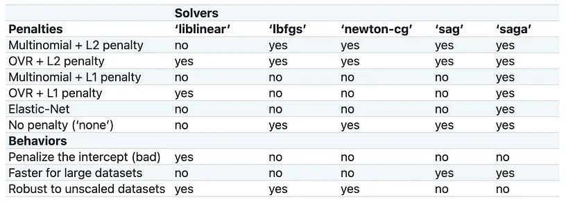
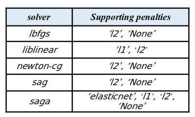
However, not all penalties are compatible with every solver. The table below summarizes the supported penalties for each solver:
Results and discussion
To accomplish our main task, we have chosen the diabetes dataset available on Kaggle.

The goal of this classification problem is to develop a model that can accurately classify patients as either diabetic or non-diabetic based on their medical information. This is a binary classification problem. This type of classification problem is important in healthcare as it can assist in the early diagnosis and treatment of diabetes, which is a chronic disease that affects millions of people worldwide.
The statistical overview of the dataset is presented below:

Before tuning the hyperparameters, we create a baseline model by fitting the classifier with default parameters.
Output:

We will use accuracy, precision, and recall as baseline metrics to compare any progress made during the optimization work. We will also examine the impact of each hyperparameter on model accuracy. In the primary model, default values were used for the solver and penalty hyperparameters.
Interestingly, the accuracy of the test data exceeded that of the train data. Moreover, we observed a precision of 0.73.
Since the choice of solver depends on the chosen penalty, we aim to select the most suitable solver based on the penalties supported by each solver in order to enhance the metrics in comparison to the initial model.
Finding the best ‘’solver” and “penalty”
At first, we start with the default value of the solver i.e. “lbfgs” and penalty = “None”:
Output:

It can be seen that the metrics of the model improved compared to the initial model.
Then we calculate the metrics for the rest of the solvers with penalty = “None”:
Output:

Similarly, it can be seen that the metrics of the model improved compared to the initial model and obtained the same metrics as the previous setting (“lbfgs” and penalty = “None”).
Now, we calculate metrics for solvers with penalty = ‘l2’:
Output:

It can be seen that these values of metrics are the same as the values of the base model.
By setting solver = “liblinear” with penalty = “l1/l2”, we calculate the metrics of the model:
Output:

Output:

It is evident that the training and testing accuracies for the L1 penalty are superior to those for the L2 penalty. Conversely, the L1 penalty’s precision value is not as high as that of the L2 penalty.
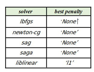
The optimal penalties for enhancing model accuracy for various solvers, based on the investigations conducted on the diabetes dataset, are displayed in the table below:
In the following, we assess the impact of various hyperparameters on the model’s accuracy to determine if they enhance its performance or not.
Examining “max_iter” parameter
In the following step, we incorporate a max_iter layer to assess its impact on the model’s accuracy. Typically, we employ the default max_iter value, which is max_iter = 100. Alternatively, we can select the maximum iteration count using the max_iter parameter, where we usually increase the value for convergence when we have an extensive amount of train data [4].
Output:

It is evident that when varying the max_iter with values of 100, 200, 500, and 1000 did not lead to any significant changes in the model’s test accuracy.
Examining “C” parameter
“C” (in the default mode is equal to 1) is a penalty term that controls the trade-off between the complexity and accuracy of a machine learning model to eliminate and adjust overfitting. A low value of “C” means that the model prefers simplicity overfitting the data well. This may lead to underfitting or misclassification of some examples. A high value of “C” means that the model tries to fit the data as well as possible, even if it means using a more complex decision boundary. This may lead to overfitting or sensitivity to noise. (A high “C” value indicates that the model gives more weight to the training data and reduces the weight assigned to the complexity penalty, and a low value of “C” indicates the model gives more weight to this complexity penalty at the cost of fitting the training data). {float, default=1.0} [4].
We aim to examine the impact of balancing the training data against the complexity penalty. To achieve this, we will set the penalty type to “l2”.
Output:

It appears that when the values of C are adjusted from 1 to 10, the model’s accuracy improves as C increases. This effectively assigns more weight to the training data compared to the complexity penalty. Furthermore, assigning a value of C higher than 10 did not result in any additional improvement in test accuracy.
Examining “tol” parameter
The parameter “tol” controls the tolerance for the stopping criterion of the algorithm. A larger value means the algorithm will stop sooner, but it may not reach the optimal solution. A smaller value means the algorithm will run longer, but it may find a better solution. However, there is a trade-off between accuracy and efficiency. {float, default=1e-4} [4].
Output:

As the value of tol rises from 0.0001 (the default value) to 10, the test accuracy diminishes. Lower values allow the algorithm more time to converge.
Examining “fit_intercept” parameter
The parameter “fit_intercept” controls whether the logistic regression model has a bias term or not. If we set fit_intercept = False, the model assumes that the data is centered around the origin, and the equation of the decision boundary will have a zero bias. The default value of “fit_intercept” is True, which means that the model will learn a non-zero bias from the data [4].
Output:

The results show that setting fit_intercept = True provides better test accuracy than setting fit_intercept = False.
Examining “intercept_scaling” parameter
The “intercept_scaling” parameter is used to reduce the effect of regularization on the intercept term. By increasing the “intercept_scaling” value, you can indeed reduce the regularization effect on the feature weight and the decision boundary width. {float, default=1} [4].
Output:
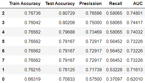
Analyzing the outcomes of different intercept_scaling values shows that the optimal accuracy is achieved for 0.2.
Examining “class_weight” parameter
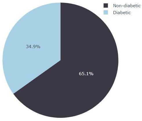
The figure above shows that the class distribution of the diabetes dataset is imbalanced.
The parameter “class_weight” adjusts the weight of each class in logistic regression. If the data has imbalanced classes, we can set class_weight = ‘balanced’, which means that the model will use inverse proportions of the class frequencies to balance the data. {dict or ‘balanced’, default=None} [4].
Output:

The results show that the ‘None’ mode exhibited greater test accuracy than the balanced mode.
Examining “random_state” parameter
The parameter “random_state” sets the seed for the random number generator in logistic regression. This ensures that the algorithm has a consistent randomness, which can be reproduced by using the same value of random_state. {int, RandomState instance, default=None} [4].
Output:

No enhancement in model test accuracy was noticed when altering the values of random_state.
Examining “multi_class” parameter
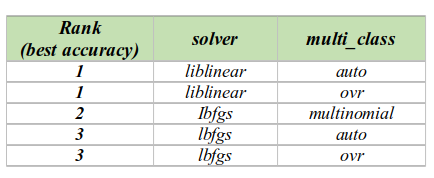
The parameter “multi_class” determines how to handle multiple classes in logistic regression. If it is ‘ovr’, the model will use a one-vs-rest strategy, which means fitting a binary model for each class. If it is ‘multinomial’, the model will use the softmax function, which means minimizing the multinomial loss over the whole probability distribution. The ‘multinomial’ option is not compatible with solver = ‘liblinear’. The default value of “multi_class” depends on the data and the solver. If the data is binary or the solver is ‘liblinear’, it will be ‘ovr’. Otherwise, it will be ‘multinomial’. {‘auto’, ‘ovr’, ‘multinomial’}, default=’auto’ [4].
Output:
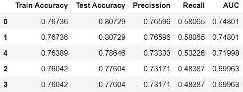
The comparison of “multi_class” results is given in the following table:
Examining “verbose” parameter
The parameter “verbose” controls the verbosity of the algorithm. It determines how many messages are displayed during the model optimization. It can be set to any positive integer value. A larger value means more messages are shown. The “verbose” option is only available for solver = ‘liblinear’, and ‘lbfgs’ [4].
Output:

The results indicate that varying values of “verbose” had no impact on enhancing the model’s test accuracy.
Examining “warm_start” parameter
The parameter “warm_start” allows us to use the previous model’s solution as the starting point for the current model. This can speed up convergence and save computation time. The default value of “warm_start” is False, which means that the model will start from scratch each time. We can set warm_start = True if we want to reuse the previous model’s learnings. Moreover, it is useless for the “liblinear” solver [4].
Output:
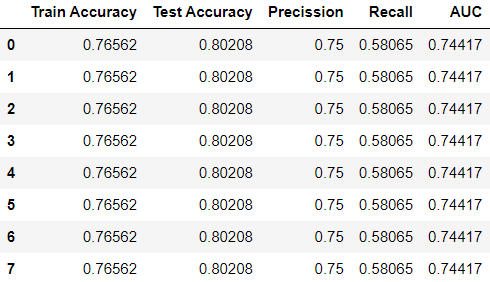
The test accuracy of the model was not affected by changing the “warm_start” to True or False for different solvers.
Examining “l1_ratio” parameter
The parameter “l1_ratio” controls the balance between ‘l1’ and ‘l2’ regularization in logistic regression.
· Setting l1_ratio = 0 is equivalent to using penalty = ‘l2’.
· Setting l1_ratio = 1 is equivalent to using penalty = ‘l1’.
· If 0 < l1_ratio < 1, the model will use a mix of l1 and l2 penalties.
The parameter “l1_ratio” is only applicable when penalty = “elasticnet” and solver= “saga” in logistic regression [4].
Output:

The comparison of the results shows that higher accuracy is provided for l1_ratio=1 > l1_ratio=0.5 > l1_ratio=0, respectively.
The best hyperparameters for the diabetes dataset were extracted from the above results and summarized in the table below:
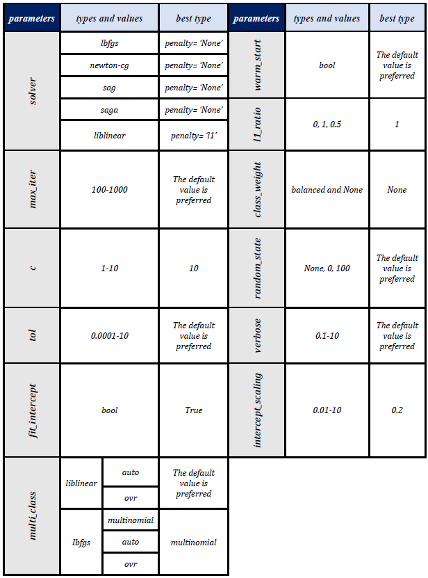
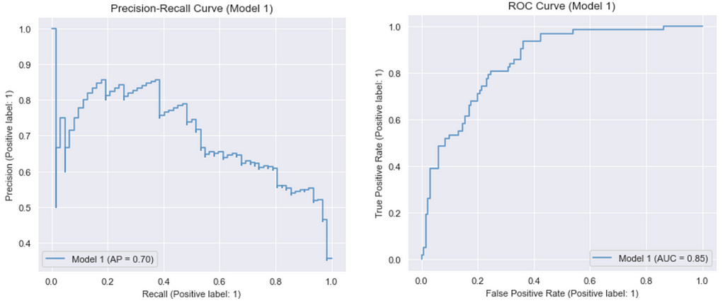
In the end, we make several models according to the above summary and compare the results with each other:
Model 1: Default hyperparameters
Output:

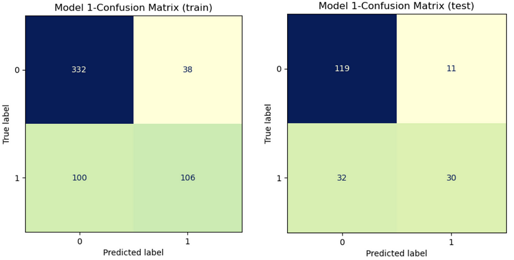
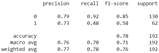
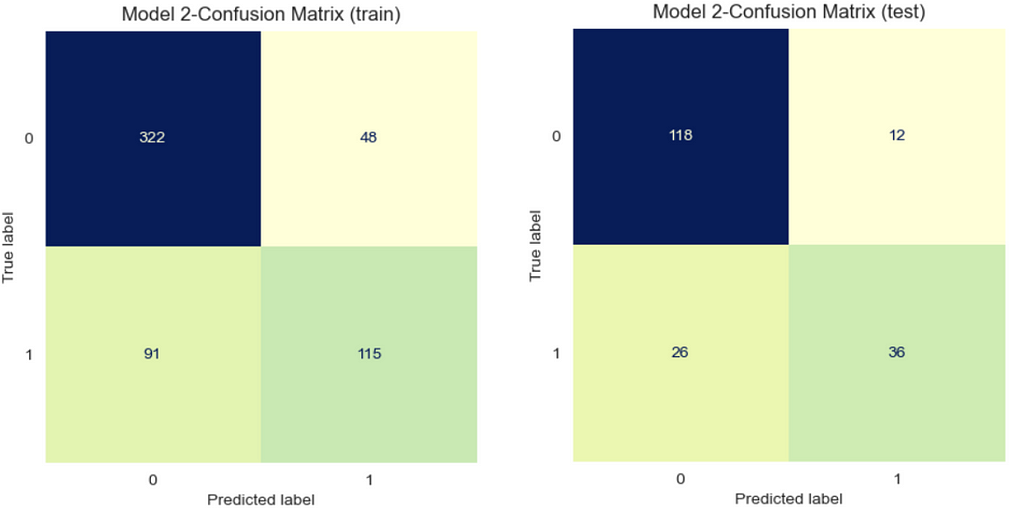
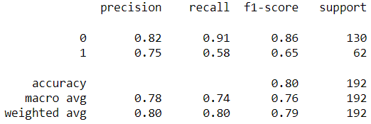
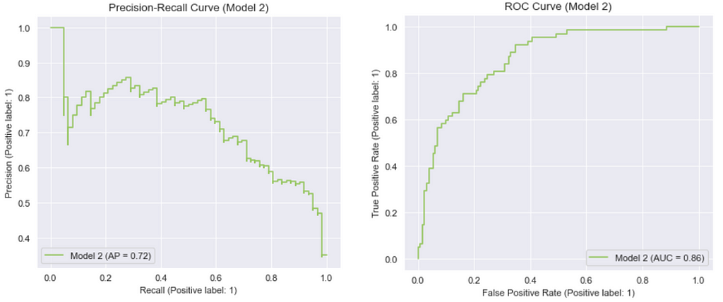
Model 2: Best hyperparameters for “liblinear” (Manually tuned)
Output:

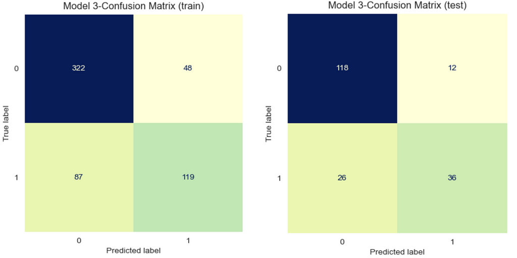
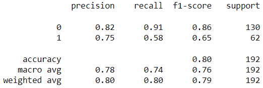
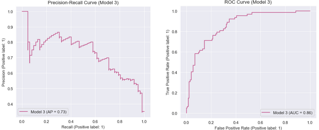
Model 3: Best hyperparameters for “lbfgs” (Manually tuned)
It is important to mention that in Model 3, the default value was used for “C”. If this value was not set accordingly, the model would experience an error.
Output:

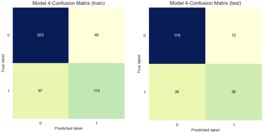
Model 4: Best hyperparameters for “newton-cg” (Manually tuned)
It is important to mention that for Model 4, the value of “C” was kept at its default setting; otherwise, the model would experience an error.
Output:

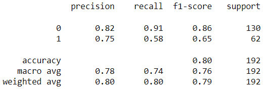
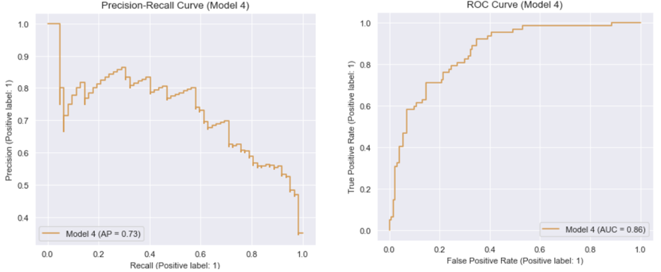
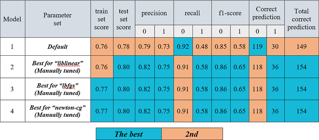
The results of the models (1–4) are summarized in the following table:
Moreover, as we mentioned earlier in this article, manual hyperparameter tuning can be a time-consuming process. However, there are several automated methods available, such as GridSearchCV and RandomizedSearchCV, which are provided by Scikit-learn [6, 7].
Conclusion
The manually tuned Models 2 through 4 exhibited improved performance in terms of accuracy, precision, recall, and F1 score on the test set in comparison to Model 1, which utilized default hyperparameters. Moreover, the classifiers in Models 2 to 4 demonstrated enhanced performance in predicting label 1 (with six more correct labels) compared to Model 1. This suggests that the classifiers in Models 2 to 4 were more effective in predicting total correct labels than the classifier in Model 1 with the default hyperparameters.
In summary, understanding the influence of hyperparameters on a model’s performance and becoming proficient in adjusting them is essential for achieving optimal results.
We hope our findings have provided you with a deeper understanding of this crucial aspect of machine learning.
The source code of this article is available on GitHub.
References
[1] https://www.geeksforgeeks.org/understanding-logistic-regression/
[2] https://www.spiceworks.com/tech/artificial-intelligence/articles/what-is-logistic-regression/
[3] https://www.blog.trainindata.com/hyperparameter-tuning-for-machine-learning/
[4] https://scikit-learn.org/stable/modules/generated/sklearn.linear_model.LogisticRegression.html
[5] https://medium.com/codex/do-i-need-to-tune-logistic-regression-hyperparameters-1cb2b81fca69
[6] https://scikit-learn.org/stable/modules/generated/sklearn.model_selection.GridSearchCV.html
[7] https://scikit-learn.org/stable/modules/generated/sklearn.model_selection.RandomizedSearchCV.html
Author: Ali Farahmandfar
Editor: Melanee
Level Up Coding
Thanks for being a part of our community! Before you go:
- 👏 Clap for the story and follow the author 👉
- 📰 View more content in the Level Up Coding publication
- 💰 Free coding interview course ⇒ View Course
- 🔔 Follow us: Twitter | LinkedIn | Newsletter
🚀👉 Join the Level Up talent collective and find an amazing job
A Comprehensive Analysis of Hyperparameter Optimization in Logistic Regression Models was originally published in Level Up Coding on Medium, where people are continuing the conversation by highlighting and responding to this story.
This content originally appeared on Level Up Coding - Medium and was authored by Melanee Group
Melanee Group | Sciencx (2023-05-21T19:06:25+00:00) A Comprehensive Analysis of Hyperparameter Optimization in Logistic Regression Models. Retrieved from https://www.scien.cx/2023/05/21/a-comprehensive-analysis-of-hyperparameter-optimization-in-logistic-regression-models/
Please log in to upload a file.
There are no updates yet.
Click the Upload button above to add an update.
