This content originally appeared on Level Up Coding - Medium and was authored by Shitanshu Bhushan
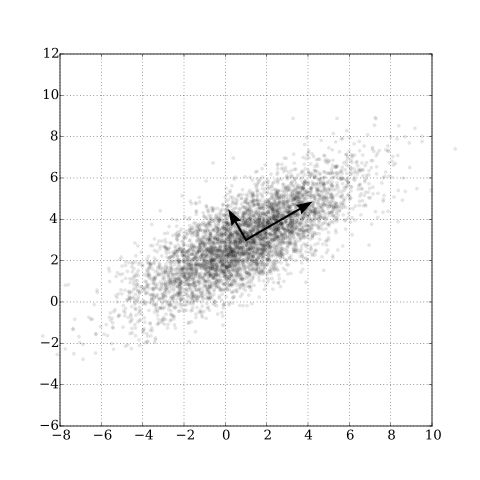
Continuing in our series of from-scratch implementations, in this article we will cover Principal Component Analysis (PCA)
What is PCA anyway ???

The above is a 28x28 dimensional image, now if we wanted to just differentiate between different variations of 8 then do we need all the 784 dimensions (considering each pixel as 1 dimension) it currently has? If we look at the degrees of freedom 8 has: it can move along X axis, it can move along Y axis, and it can also be rotated, we can basically encode all the information in just 3-dimensions. So we should be able to represent the above data in just 3 dimensions instead of 784 but how do we do that? This is where PCA comes in!
PCA is a mathematical algorithm that reduces the dimension of the data while retaining as much information as possible. Given a set of observations in a space of dimension D, the goal of PCA is to find a subspace K, K<D, such that it captures most of the variability of our data.
It can be thought of as a projection of all these points from the higher dimension D to the lower dimension K. PCA can be described as:
- Maximizing the variance of the projection, OR
- Minimizing the squared approximation error
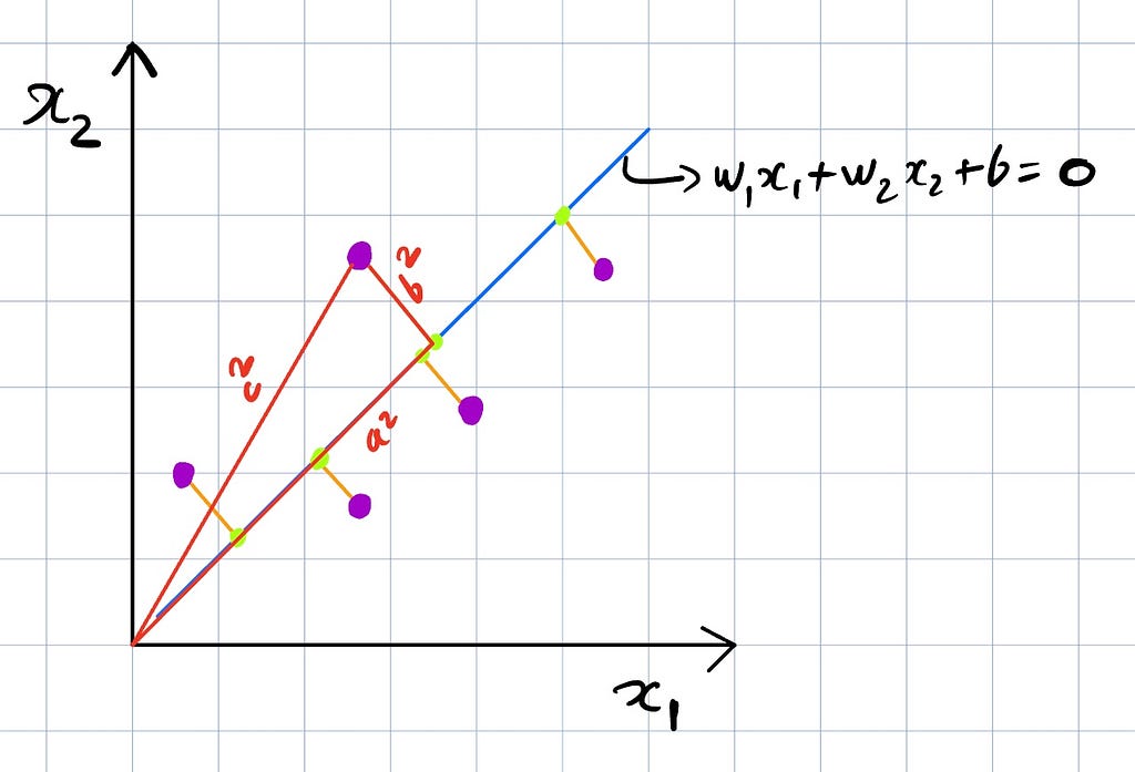
Let’s look at the above image as an example, we have a 2-dimensional space and we want to project these points in a 1-dimensional space, which would be a line. Considering the mean at origin, b² is the projection error and a² is the variance, with a constant c², the goal of this projection then can be seen as either minimizing b² (projection error) or maximizing a² (variance), which is what we just highlighted PCA can be described as.
Okay now let’s see some maths behind PCA,
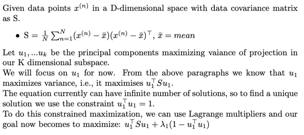
To maximize the above equation, we need to take its derivative and set it to zero. Doing that we find that

Thus, ƛ₁ is the largest eigenvalue of S and u₁ is the corresponding eigenvector. We can repeat the above to find the K eigenvectors corresponding to the K largest eigenvalues.
A useful use case of PCA can be when you have highly linearly correlated data. PCA can help remove this collinearity as all the principal components are orthogonal to each other.
So to implement PCA we just need to find the eigenvalues and eigenvectors of the covariance matrix of the data. An important point to note is that the data should be normalized before finding the covariance matrix.
Using the Fashion MNIST dataset we used for logistic regression we got an accuracy of around 76%. The data currently has 784 dimensions but do we really need all those dimensions? let’s see if we can use PCA to reduce the dimensionality of the data and improve the accuracy.
Before we begin our implementation, let’s see what performance we get using PCA from sklearn,
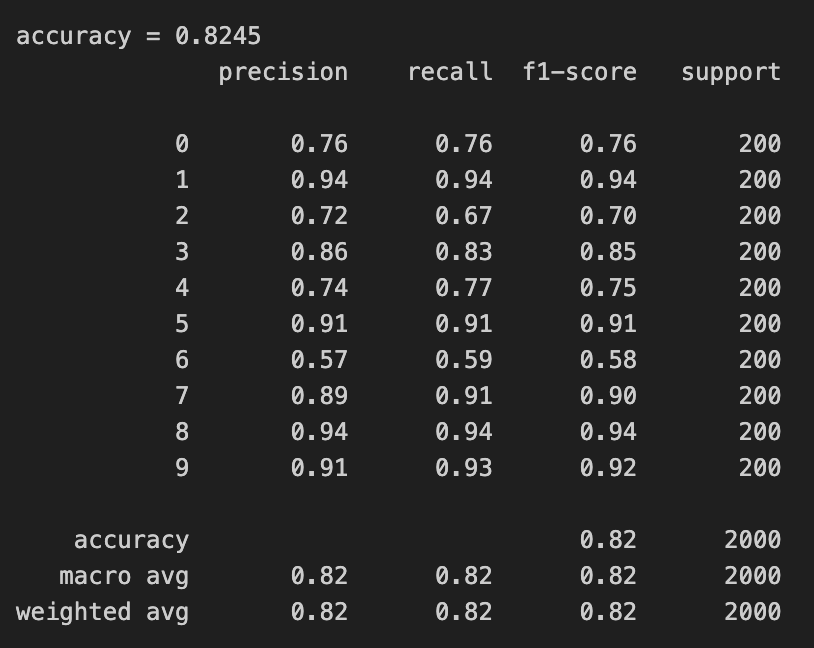
We reduced the dimensionality to 50 from 784 and we can see that our accuracy went up and also the time to train went down as we now have a much smaller dimension data. Okay so now let’s implement this from scratch
From-Scratch Implementation
The steps for this implementation are relatively simple:
- First, normalize the data. This helps deal with non-gaussian data issues.
- Find the covariance matrix
- Find the eigenvalues and eigenvectors of the covariance matrix
- Rearrange the eigenvalues and eigenvectors and select the top K principal components
Let’s see what this looks like in code:
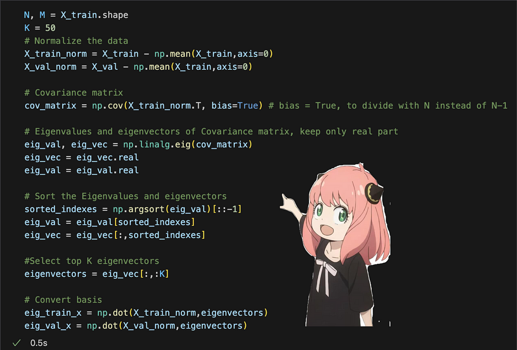
We follow all the steps I laid out above and then project our data into the smaller dimension subspace at the end.

From the image above, we can see that with just 34 principal components we can explain 95% variance in our data which shows why PCA can be a useful tool as we didn’t really need all 784 dimensions that our data has to begin with.
We can also visualize these top K eigenvectors and see what they are focusing on,

We can see that the first few eigenvectors are focusing on shirts and pants. Some are focusing on the variation in shoulders or sleeves, we can also see variations in boots, etc. Now let’s see how our implementation performs as compared to sklearn:
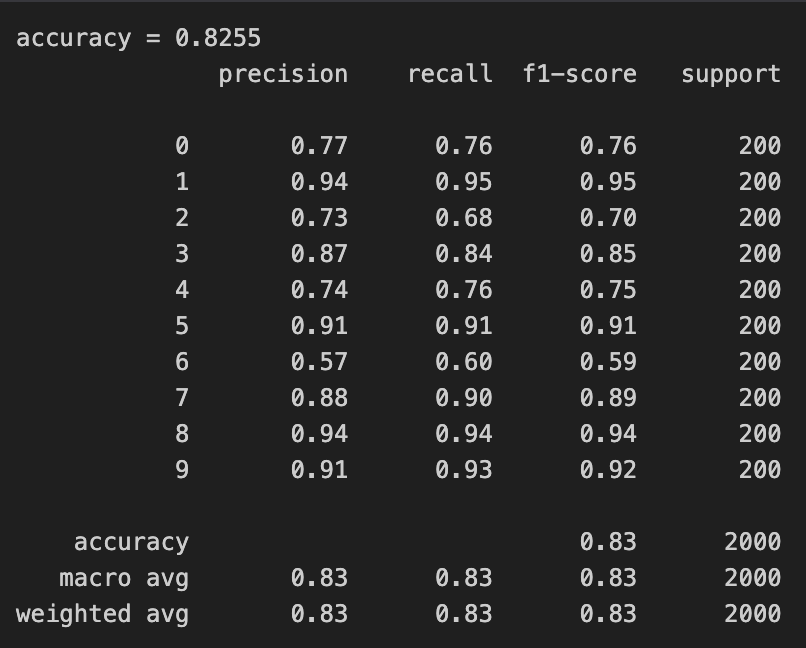
We can see that our implementation performs similar to using sklearn and our implementation also took less time to train but that difference wasn’t too significant.
Summary
As we saw above, implementing PCA is relatively simple and is easy to match sklearn’s output. PCA is mostly used for dimensionality reduction and visualization but it can be used for other cases too, Eigenfaces is a famous example where PCA was used for face detection which shows how powerful the tool is. There are many situations where PCA fails though like non-gaussian data, non-linear manifolds, etc and in such cases we are better off using other methods like ISOMAP, etc. Even for visualization, there are other tools like t-SNE which is used commonly to visualize clusters.
All the code for this can be found at — PCA from scratch
Principal Component Analysis: Reducing dimensionality from scratch was originally published in Level Up Coding on Medium, where people are continuing the conversation by highlighting and responding to this story.
This content originally appeared on Level Up Coding - Medium and was authored by Shitanshu Bhushan
Shitanshu Bhushan | Sciencx (2024-06-18T20:01:24+00:00) Principal Component Analysis: Reducing dimensionality from scratch. Retrieved from https://www.scien.cx/2024/06/18/principal-component-analysis-reducing-dimensionality-from-scratch/
Please log in to upload a file.
There are no updates yet.
Click the Upload button above to add an update.
