
This content originally appeared on Level Up Coding - Medium and was authored by Satyajit Chaudhuri
Time Series Forecasting is no more a domain for Statistical Algorithms only. Traditional Machine learning Models have already shown significant success in Time Series Forecasting tasks and can become very significant when you are dealing with external indicators(promotions, discounts, holidays and a lot more).
My last article “Can Machine Learning Outperform Statistical Models for Time Series Forecasting?” has gained significant attention from the readers. Also there has been some wonderful questions about the MLForecast Library by the Nixtla team. In this article, I will address some of those questions, providing a detailed walkthrough of the library and demonstrating how to use it for your time series data. Let’s dive into forecasting.

This article will broadly discuss the following:
- Introduction
2. Understanding MLForecast
3. Feature Generation
4. Implementation Guide
5. Forecasting Process
6. Case Study
7. Conclusion
The MLForecast Library
MLForecast is a powerful library within the Nixtla ecosystem designed for time series forecasting using machine learning models. MLForecast allows users to define models, features (including lags, transformations on lags, and date features), and target transformations. This library offers several key features and capabilities:
- MLForecast offers a framework for performing time series forecasting using machine learning models.
- It has the option to scale to massive amounts of data using remote clusters.
- MLForecast is compatible with models that follow the scikit-learn API, making it highly flexible and allowing seamless integration with a wide variety of machine learning algorithms
- MLForecast is engineered to execute tasks rapidly, which is crucial when handling large datasets and complex models .
- It is capable of horizontal scaling using distributed computing frameworks such as Spark, Dask, and Ray. This feature enables it to efficiently process massive datasets by distributing the computations across multiple nodes in a cluster, making it ideal for large-scale time series forecasting tasks .
MLForecast ensures high performance and scalability
The MLForecast is engineered to execute tasks rapidly, which is crucial when handling large datasets and complex models.
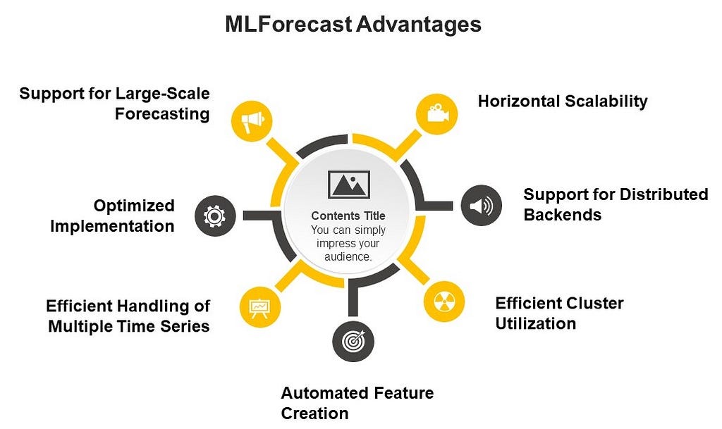
Horizontal Scalability: MLForecast is capable of horizontal scaling using distributed computing frameworks such as Spark, Dask, and Ray. This feature enables it to efficiently process massive datasets by distributing the computations across multiple nodes in a cluster, making it ideal for large-scale time series forecasting tasks.
Support for Distributed Backends: MLForecast can automatically dispatch to the corresponding backend based on the input data type:
- If you provide a pandas dataframe, it will run locally. Here you can set n_jobs>1 to use multiprocessing on your local machine.
- If you provide a spark dataframe, it will run in your cluster. In this case, n_jobs will automatically be set to 1 to avoid nested parallelism (spark handles the parallelism here).
Efficient Cluster Utilization: To maximize the utilization of your cluster when using Spark, you should ensure that you have at least as many partitions as executors (or a multiple of them) so that Spark can schedule at least one task per executor.
Automated Feature Creation: MLForecast provides automated feature creation for time series forecasting, which can significantly speed up the model development process.
Efficient Handling of Multiple Time Series: MLForecast is designed to handle multiple time series efficiently. It uses a single (global) model for all series, which is usually faster and can perform better than training separate models for each series.
Optimized Implementation: The core functionality of MLForecast is implemented using efficient libraries and algorithms.
Support for Large-Scale Forecasting: MLForecast is designed to handle large-scale forecasting tasks. For example, it can efficiently process datasets with millions of time series.
It’s worth noting that while these features contribute to high performance and scalability, the actual performance will depend on various factors including the specific models used, the size and complexity of the dataset, and the available computational resources.
For the most up-to-date and detailed information on MLForecast’s performance optimizations, you might want to check the latest documentation or reach out to the Nixtla community directly.
How MLForecast Forecasts?
MLForecast carries out forecasting using a recursive strategy by default. This means it predicts one step at a time, using the predictions from previous steps as inputs for future steps.
Here’s a detailed explanation of how MLForecast performs forecasting at each step:
- Initial Setup: When you create an MLForecast object, you specify the models, frequency, lags, and other parameters.
- Feature Creation: MLForecast automatically creates features based on the lags and lag transforms you’ve specified.
- Model Training: During the fit process, MLForecast trains the specified models on the historical data, using the created features .
- Forecasting Process: When you call the predict method, it generates the forecast. This step will be discussed in the more details in the next sub section.
- Handling Multiple Models: If you’ve specified multiple models, MLForecast will repeat the forecasting process for each model.
- Output: The final output is a DataFrame containing the predictions for each specified model across the forecast horizon.
The predict method in MLForecast follows these steps for each forecast horizon:
a. For the first step:
- It uses the actual historical data to create the lagged features.
- The model makes a prediction for this step using these features.
b. For subsequent steps:
- It uses a combination of historical data and previously predicted values to create the lagged features .
- For example, if you’re predicting the second step and you have a lag of 1, it will use the prediction from the first step as the lag 1 feature .
- The model then makes a prediction for this step using these updated features.
c. This process continues for each step in the forecast horizon in a recursive way, always using the most recent predictions to update the lagged features.
It’s important to note that this recursive strategy can lead to error accumulation over longer forecast horizons, as each step’s prediction is based on previous predictions rather than actual values.
MLForecast also supports a direct multi-step forecasting approach, where separate models are trained for each step in the forecast horizon. This can be activated by setting the max_horizon parameter in the fit method. In this case:
- MLForecast trains separate models for each step in the forecast horizon .
- When predicting, it uses the appropriate model for each step, which can potentially reduce error accumulation over longer horizons .
Remember, the exact behavior may vary depending on the specific models and parameters you’re using. The recursive strategy is the default, but you have the flexibility to adjust this based on your specific forecasting needs.
A detailed example of forecasting using MLForecast will be discussed in a coming section.
Feature Generation for ML Forecasting
MLForecast is designed to work with a variety of machine learning algorithms. Unlike Statistical algorithms, the ML algorithms do not automatically understand the temporal dependence of the data. It relies on the features given to the model as inputs during the training phase, to learn more about the time series. In this section we will discuss the feature generation steps along-with examples for practical implementation.
- Lags: MLForecast allows you to specify lag values to be used as regressors. These are defined when creating an MLForecast object using the lags parameter.
- Lag Transforms: MLForecast also allows you to apply transformations to lagged features. This is done using the lag_transforms parameter. MLForecast offers several built-in lag transforms that can be applied to lagged features. These transforms can be categorized into three main groups:
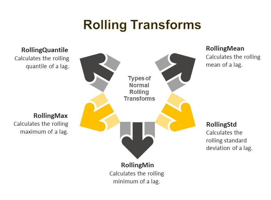
2.1 Rolling Transforms:
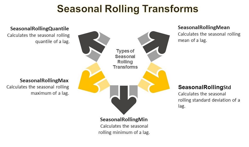
2.2 Seasonal Rolling Transforms:
2.3. Expanding Transform:
- ExpandingMean: Calculates the expanding mean of a lag.
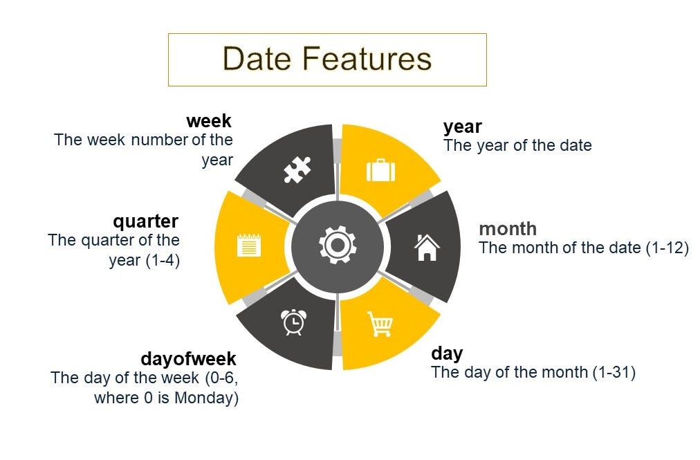
3. Date Features: As shown in the example above, you can also specify date features to be generated automatically . These are computed from the dates and can include attributes like year, month, day, day of week, quarter, and week.
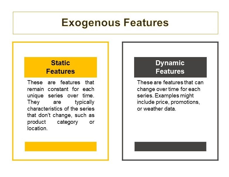
4. Exogenous Features: MLForecast supports both static and dynamic exogenous features. You can transform exogenous features using the transform_exog function.
5. Target Transforms
Target transforms in MLForecast serve multiple crucial purposes in time series forecasting, primarily aimed at improving model performance and data characteristics . These transformations can help achieve stationarity, which is essential for many forecasting models, by removing trends and stabilizing variance . They also facilitate normalization, handling of non-linear relationships, and can be tailored to different types of data . A key advantage of using target transforms in MLForecast is the automatic handling of inverse transformations during prediction, simplifying the forecasting process . The flexibility to chain multiple transformations allows for customized approaches to various forecasting challenges . While transforms like differencing (e.g., `Differences([1])`) are commonly used to remove trends, others like `LocalStandardScaler` can standardize each series individually . The choice of transformation should be based on the specific characteristics of your data and the requirements of your forecasting task, often requiring experimentation to find the most effective approach .
AutoDifferences is a more advanced and automated approach to differencing. It automatically determines the optimal number of differences to apply to each group (time series) in your data. It uses statistical tests to determine if a series is stationary, and if not, it applies differencing until stationarity is achieved or the maximum number of differences is reached. The max_diffs parameter sets the maximum number of differences that can be applied .
e.g.,
from mlforecast import MLForecast
from coreforecast.scalers import AutoDifferences
import lightgbm as lgb

# Create an MLForecast instance with AutoDifferences
fcst = MLForecast(
    models=[lgb.LGBMRegressor()],
    freq='D',
    lags=[1, 7, 14],
    target_transforms=[AutoDifferences(max_diffs=2)]
)

# Fit the model and make predictions
fcst.fit(train_data)
predictions = fcst.predict(horizon=30)
Setting max_diffs=2 gives AutoDifferences the flexibility to apply either first-order or second-order differencing, depending on what's needed to achieve stationarity for each series. Going beyond second-order differencing (i.e., max_diffs > 2) is rarely necessary and can lead to over-differencing, which can introduce unnecessary complexity and potentially harm forecast accuracy.
A Sample Feature Generation for different Time Scales
For Quarterly Data:
from mlforecast import MLForecast
from mlforecast.lag_transforms import RollingMean, ExpandingMean

fcst = MLForecast(
    models=[],  # Add your models here
    freq='Q',   # Quarterly frequency
    lags=[1, 4],  # Lag of 1 quarter and 1 year
    lag_transforms={
        1: [ExpandingMean()],
        4: [RollingMean(window_size=4)]  # Rolling mean over the past year
    },
    date_features=['quarter']
)
For Monthly Data:
fcst = MLForecast(
    models=[],  # Add your models here
    freq='M',   # Monthly frequency
    lags=[1, 12],  # Lag of 1 month and 1 year
    lag_transforms={
        1: [ExpandingMean()],
        12: [RollingMean(window_size=12)]  # Rolling mean over the past year
    },
    date_features=['month']
)
For Weekly Data:
fcst = MLForecast(
    models=[],  # Add your models here
    freq='W',   # Weekly frequency
    lags=[1, 4, 52],  # Lag of 1 week, 1 month, and 1 year
    lag_transforms={
        1: [ExpandingMean()],
        4: [RollingMean(window_size=4)],  # Rolling mean over the past month
        52: [RollingMean(window_size=52)]  # Rolling mean over the past year
    },
    date_features=['week']
)
For Daily Data:
fcst = MLForecast(
    models=[],  # Add your models here
    freq='D',   # Daily frequency
    lags=[1, 7, 30, 365],  # Lag of 1 day, 1 week, 1 month, and 1 year
    lag_transforms={
        1: [ExpandingMean()],
        7: [RollingMean(window_size=7)],   # Rolling mean over the past week
        30: [RollingMean(window_size=30)], # Rolling mean over the past month
        365: [RollingMean(window_size=365)] # Rolling mean over the past year
    },
    date_features=['dayofweek', 'month']
)
For Hourly Data:
fcst = MLForecast(
    models=[],  # Add your models here
    freq='H',   # Hourly frequency
    lags=[1, 24, 168, 720],  # Lag of 1 hour, 1 day, 1 week, and 1 month
    lag_transforms={
        1: [ExpandingMean()],
        24: [RollingMean(window_size=24)],   # Rolling mean over the past day
        168: [RollingMean(window_size=168)], # Rolling mean over the past week
        720: [RollingMean(window_size=720)]  # Rolling mean over the past month
    },
    date_features=['hour', 'dayofweek']
)
Forecasting Models used in MLForecast
MLForecast is designed to work with various machine learning models that follow the scikit-learn API. Some of the common models available in this are:
- Linear Regression: This is a basic algorithm that’s often used as a baseline model. It’s included in many examples in the MLForecast documentation.
- LightGBM: This is a gradient boosting framework that uses tree-based learning algorithms. It is designed for speed and efficiency. It uses a novel technique of leaf-wise tree growth instead of the traditional level-wise, improving accuracy and reducing overfitting. Suitable for large datasets, it supports parallel and GPU learning, making it a powerful tool for high-performance machine learning tasks.
- XGBoost: Extreme Gradient Boosting is a scalable and efficient gradient boosting framework. It uses advanced regularization techniques to prevent overfitting and supports parallel and distributed computing. Known for its speed and performance, XGBoost is widely used in machine learning competitions and real-world applications, making it a popular choice for predictive modeling and data analysis.
- Random Forest: Random Forest is a bagging based ensemble learning method that constructs multiple decision trees during training. It merges their predictions to improve accuracy and control overfitting. By averaging multiple trees, it enhances performance and reduces variance. Robust to noisy data and effective for classification and regression tasks, Random Forest is widely used for its simplicity and strong predictive power.
Now if you do not happen to find a suitable model for your task. You can also write your own model.
Here’s a step-by-step guide on how to do this:
First, you need to create a custom model class that inherits from sklearn.base.BaseEstimator and implements the required methods. Here's a basic structure:
from sklearn.base import BaseEstimator, RegressorMixin
from sklearn.utils.validation import check_X_y, check_array, check_is_fitted

class CustomModel(BaseEstimator, RegressorMixin):
    def __init__(self, param1=1, param2=1):
        self.param1 = param1
        self.param2 = param2

    def fit(self, X, y):
        # Check that X and y have correct shape
        X, y = check_X_y(X, y)
        # Store the classes seen during fit
        self.classes_ = unique_labels(y)

        # Your model fitting logic here

        # Return the classifier
        return self

    def predict(self, X):
        # Check is fit had been called
        check_is_fitted(self)
        # Input validation
        X = check_array(X)

        # Your prediction logic here

        return y_pred
Once you have defined your custom model, you can use it within MLForecast just like any other scikit-learn compatible mode.
from mlforecast import MLForecast
from your_module import CustomModel

mlf = MLForecast(
    models=[CustomModel()],  # Use your custom model here
    freq='D',  # Frequency of the data - 'D' for daily frequency
    lags=[1, 2, 3],  # Lag features to use
    date_features=['dayofweek', 'month'],  # Date-based features
)
You can then use this MLForecast instance with your custom model for fitting and prediction, just as you would with any other model :
# Fit the model
mlf.fit(df)

# Make predictions
predictions = mlf.predict(horizon=7)
It’s important to note that your custom model should implement at least the fit and predict methods to be compatible with MLForecast 1. The fit method should take X (features) and y (target) as inputs and return self. The predict method should take X as input and return predictions .
Also, make sure your custom model can handle the features that MLForecast generates, including lag features and date features 2.
Remember, MLForecast is designed to work with regression models, so your custom model should be appropriate for regression tasks.
If you need to pass custom parameters to the fit function of your model, you might need to implement a custom training approach. It’s suggested to first determine the best parameters and then use them in the regular MLForecast.fit method.
Now Let’s put the steps together.
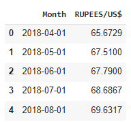
In this experimental part we are using USD — INR Monthly conversion values (Indian Rupees/ US Dollars) which can be downloaded from here. The data is for the time period April 2018 to March 2024.
Let’s install the mlforecast
#This will also install collected packages: window-ops, utilsforecast, mlforecast
!pip install mlforecast
Let’s download the required libraries
import seaborn as sns
import matplotlib.pyplot as plt
import numpy as np
from mlforecast import MLForecast
from mlforecast.target_transforms import Differences
from numba import njit
import lightgbm as lgb
import xgboost as xgb
from sklearn.linear_model import LinearRegression
from sklearn.ensemble import RandomForestRegressor
from statsmodels.tsa.seasonal import seasonal_decompose
from mlforecast import MLForecast
from mlforecast.lag_transforms import (
    RollingMean, RollingStd, RollingMin, RollingMax, RollingQuantile,
    SeasonalRollingMean, SeasonalRollingStd, SeasonalRollingMin,
    SeasonalRollingMax, SeasonalRollingQuantile,
    ExpandingMean
)
from coreforecast.scalers import AutoDifferences
Now we would be reading our data to a dataframe.
file_path = "USD-INR.csv"
df = pd.read_csv(file_path)
df['Month'] = pd.to_datetime(df['Month'])
df = df.set_index('Month').resample('MS').mean()
df = df.interpolate() #to interpolate and fill missing values
df.reset_index(inplace=True)
print(df.head())
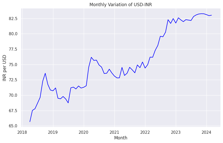
Let’s visualize our data.
sns.set(style="darkgrid")
plt.figure(figsize=(10, 6))
sns.lineplot(x="Month", y='RUPEES/US$', data=df, color='bLUE')
plt.title('Monthly Variation of USD-INR')
plt.xlabel('Month')
plt.ylabel('INR per USD')
plt.show()
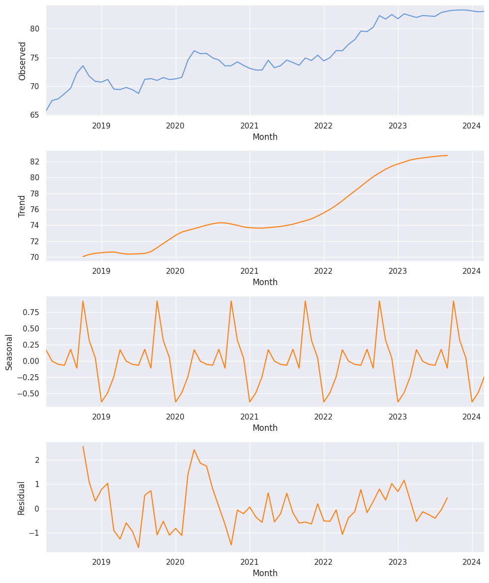
Also, we wish to check the seasonal decomposition of that data.
result = seasonal_decompose(df['RUPEES/US$'], model='additive')

fig, (ax1, ax2, ax3, ax4) = plt.subplots(4, 1, figsize=(10, 12))

result.observed.plot(ax=ax1, color="#69d")
ax1.set_ylabel('Observed')

result.trend.plot(ax=ax2, color='#ff7f0e')
ax2.set_ylabel('Trend')

result.seasonal.plot(ax=ax3, color='#ff7f0e')
ax3.set_ylabel('Seasonal')

result.resid.plot(ax=ax4, color='#ff7f0e')
ax4.set_ylabel('Residual')

plt.tight_layout()
plt.show()
Now for the MLForecast, we need three columns:
unique_id : The unique_id column is used to identify different time series within your dataset. - It can be a string, integer, or category type.
- It represents an identifier for each series in your data.
- This is particularly useful when you’re working with multiple time series in the same dataset.
ds (datestamp): The ds column represents the time component of your time series data. - It should be in a format that Pandas can interpret as a date or timestamp.
- Ideally, it should be in the format YYYY-MM-DD for a date or YYYY-MM-DD HH:MM:SS for a timestamp.
- This column is crucial for MLForecast to understand the temporal aspect of your data.
y (target variable): The y column contains the actual values you want to forecast. - It should be numeric.
- This is the measurement or quantity that you’re trying to predict.
df = pd.DataFrame({'unique_id':[1]*len(df),
        'ds': df["Month"], "y":df['RUPEES/US$']})
Let’s do the Train-test split
#Train-Test Split
train_size = int(len(df) * 0.8)
train, test = df.iloc[:train_size], df.iloc[train_size:]

print(f'Train set size: {len(train)}')
print(f'Test set size: {len(test)}')
Train set size: 57
Test set size: 15
Now time for the model building-
models = [LinearRegression(),  # Simple linear regression model
    lgb.LGBMRegressor(verbosity=-1),  # LightGBM regressor with verbosity turned off
    xgb.XGBRegressor(),  # XGBoost regressor with default parameters
    RandomForestRegressor(random_state=0),  # Random Forest regressor with fixed random state for reproducibility
]
fcst = MLForecast(
    models=models,  # List of models to be used for forecasting
    freq='MS',  # Monthly frequency, starting at the beginning of each month
    lags=[1,3,5,7,12],  # Lag features: values from 1, 3, 5, 7, and 12 time steps ago
    lag_transforms={
        1: [  # Transformations applied to lag 1
            RollingMean(window_size=3),  # Rolling mean with a window of 3 time steps
            RollingStd(window_size=3),  # Rolling standard deviation with a window of 3 time steps
            RollingMin(window_size=3),  # Rolling minimum with a window of 3 time steps
            RollingMax(window_size=3),  # Rolling maximum with a window of 3 time steps
            RollingQuantile(p=0.5, window_size=3),  # Rolling median (50th percentile) with a window of 3 time steps
            ExpandingMean()  # Expanding mean (mean of all previous values)
        ],
        6:[  # Transformations applied to lag 6
            RollingMean(window_size=6),  # Rolling mean with a window of 6 time steps
            RollingStd(window_size=6),  # Rolling standard deviation with a window of 6 time steps
            RollingMin(window_size=6),  # Rolling minimum with a window of 6 time steps
            RollingMax(window_size=6),  # Rolling maximum with a window of 6 time steps
            RollingQuantile(p=0.5, window_size=6),  # Rolling median (50th percentile) with a window of 6 time steps
        ],
        12: [  # Transformations applied to lag 12 (likely for yearly seasonality)
            SeasonalRollingMean(season_length=12, window_size=3),  # Seasonal rolling mean with 12-month seasonality and 3-month window
            SeasonalRollingStd(season_length=12, window_size=3),  # Seasonal rolling standard deviation with 12-month seasonality and 3-month window
            SeasonalRollingMin(season_length=12, window_size=3),  # Seasonal rolling minimum with 12-month seasonality and 3-month window
            SeasonalRollingMax(season_length=12, window_size=3),  # Seasonal rolling maximum with 12-month seasonality and 3-month window
            SeasonalRollingQuantile(p=0.5, season_length=12, window_size=3)  # Seasonal rolling median with 12-month seasonality and 3-month window
        ]
    },
    date_features=['year', 'month', 'quarter'],  # Extract year, month, and quarter from the date as features
    target_transforms=[Differences([1])])  # Apply first-order differencing to the target variable
Before we proceed…
Lets have a look at our processed data after all the features are added.
preprocessed_df = fcst.preprocess(train)
print(preprocessed_df)
The output of the preprocessing steps is embedded above.
In the next step we proceed to generate the predictions.
fcst.fit(train_)
# Fits the MLForecast model to the training data
# This trains all specified models (LinearRegression, LGBMRegressor, XGBRegressor, RandomForestRegressor)
# and prepares the feature engineering pipeline

ml_prediction = fcst.predict(len(test_))
# Generates predictions for a horizon equal to the length of the test set
# Returns a DataFrame with predictions from all models

ml_prediction.rename(columns={'ds': 'Month'}, inplace=True)
# Renames the 'ds' column (default name for date/time column in MLForecast) to 'Month'
# This is done in-place, modifying the original DataFrame

fcst_result = test.copy()
# Creates a copy of the test DataFrame to store the results
# This preserves the original test data while allowing us to add predictions

fcst_result.set_index("Month", inplace=True)
# Sets the 'Month' column as the index of the fcst_result DataFrame
# This is done in-place, modifying the DataFrame

fcst_result["LinearRegression_fcst"]=ml_prediction["LinearRegression"].values
# Adds a new column 'LinearRegression_fcst' to fcst_result
# Populates it with the predictions from the LinearRegression model

fcst_result["LGBM_fcst"]=ml_prediction["LGBMRegressor"].values
# Adds a new column 'LGBM_fcst' to fcst_result
# Populates it with the predictions from the LGBMRegressor model

fcst_result["XGB_fcst"]=ml_prediction["XGBRegressor"].values
# Adds a new column 'XGB_fcst' to fcst_result
# Populates it with the predictions from the XGBRegressor model

fcst_result["RandomForest_fcst"]=ml_prediction["RandomForestRegressor"].values
# Adds a new column 'RandomForest_fcst' to fcst_result
# Populates it with the predictions from the RandomForestRegressor model

fcst_result.head()
# Displays the first five rows of the fcst_result DataFrame
# This allows you to see a preview of the results, including the actual values and predictions from all models
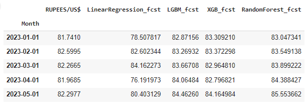
Now the results generated are stored in the dataframe fcst_result.
We can then define a function to evaluate the performance of these models. You can read more about accuracy metrices for time series forecasting in this article.
#Defining a function to calculate the error metrics
def calculate_error_metrics(actual_values, predicted_values):
    actual_values = np.array(actual_values)
    predicted_values = np.array(predicted_values)

    metrics_dict = {
        'MAE': np.mean(np.abs(actual_values - predicted_values)),  # Mean Absolute Error
        'RMSE': np.sqrt(np.mean((actual_values - predicted_values)**2)),  # Root Mean Square Error
        'MAPE': np.mean(np.abs((actual_values - predicted_values) / actual_values)) * 100}  # Mean Absolute Percentage Error

    result_df = pd.DataFrame(list(metrics_dict.items()), columns=['Metric', 'Value'])
    return result_df

# Extracting actual values from the result DataFrame
actuals = fcst_result['RUPEES/US$']

# Dictionary to store error metrics for each model
error_metrics_dict = {}

# Calculating error metrics for each model's predictions
for col in fcst_result.columns[1:]:  # Iterating through prediction columns (skipping the first column which is likely the actual values)
    predicted_values = fcst_result[col]
    error_metrics_dict[col] = calculate_error_metrics(actuals, predicted_values)['Value'].values  # Extracting 'Value' column

# Creating a DataFrame from the error metrics dictionary
error_metrics_df = pd.DataFrame(error_metrics_dict).T.reset_index()
error_metrics_df.columns = ['Model', 'MAE', 'RMSE', 'MAPE']  # Renaming columns for clarity
print(error_metrics_df)
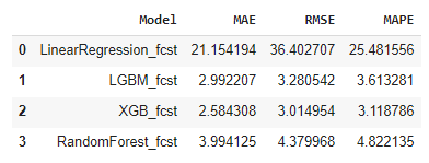
This demonstrates that the model performs well with this data. It’s important to note that, unlike the previous article, this study does not compare the ML models with other statistical or deep learning models. The primary purpose of this article is to serve as a reference for incorporating MLForecast into your forecasting toolkit.
Conclusion
In this article, we have explored the MLForecast library, a powerful tool within the Nixtla ecosystem designed for time series forecasting using machine learning models. We discussed its key features, capabilities, and the steps involved in implementing MLForecast for your forecasting needs. By providing automated feature creation, efficient handling of multiple time series, and support for large-scale forecasting, MLForecast stands out as a robust solution for time series analysis. While this study did not compare ML models with other statistical or DL models, it serves as a comprehensive reference for integrating MLForecast into your forecasting workflow. As machine learning continues to evolve, tools like MLForecast will play an increasingly significant role in enhancing the accuracy and efficiency of time series forecasting.
How to MLForecast your Time Series Data! was originally published in Level Up Coding on Medium, where people are continuing the conversation by highlighting and responding to this story.
This content originally appeared on Level Up Coding - Medium and was authored by Satyajit Chaudhuri
Satyajit Chaudhuri | Sciencx (2024-07-14T17:24:20+00:00) How to MLForecast your Time Series Data!. Retrieved from https://www.scien.cx/2024/07/14/how-to-mlforecast-your-time-series-data/
Please log in to upload a file.
There are no updates yet.
Click the Upload button above to add an update.