This content originally appeared on HackerNoon and was authored by Computational Technology for All
:::info Authors:
(1) Xiaofan Yu, University of California San Diego, La Jolla, California, USA (x1yu@ucsd.edu);
(2) Anthony Thomas, University of California San Diego, La Jolla, California, USA (ahthomas@ucsd.edu);
(3) Ivannia Gomez Moreno, CETYS University, Campus Tijuana, Tijuana, Mexico (ivannia.gomez@cetys.edu.mx);
(4) Louis Gutierrez, University of California San Diego, La Jolla, California, USA (l8gutierrez@ucsd.edu);
(5) Tajana Šimunić Rosing, University of California San Diego, La Jolla, USA (tajana@ucsd.edu).
:::
Table of Links
8 Evaluation of LifeHD semi and LifeHDa
9 Discussions and Future Works
10 Conclusion, Acknowledgments, and References
7 EVALUATION OF LIFEHD
7.1 System Implementation
We implement LifeHD with Python and PyTorch [43] and deploy it on three standard edge platforms: Raspberry Pi (RPi) Zero 2 W [3], Raspberry Pi 4B [2], and Jetson TX2 module [1]. The selection of edge platforms represent three tiers with small, medium and abundant resources.
\ RPi Zero 2 W has a 1GHz quad-core Cortex-A53 CPU and 512MB SDRAM. RPi 4B enjoys a 1.8GHz quad-core Cortex-A72 CPU and 4GB SDRAM. The Jetson TX platform is equipped with a dual-core NVIDIA Denver 2 CPU, a quad-core ARM Cortex-A57 MPCore, an NVIDIA Pasca family GPU with 256 NVIDIA CUDA cores, and 8GB RAM. We measure the training latency per batch and the energy consumption using the Hioki 3334 powermeter [19].
\ We are aware that all NN-based feature extractors can be pruned and quantized to attain more efficient deployment on edge platforms [11], same for the NN-based baselines we compare to [13, 14]. However, NN model compression is not the primary focus of LifeHD. Existing compression techniques [26, 39] can be applied directly to the feature extractor in LifeHD. We leave LifeHD with acceleration design and emerging hardware deployment for future works.
7.2 Experimental Setup
We conduct comprehensive experiments to evaluate LifeHD on three typical edge scenarios. All three scenarios incorporate continuous data streams and expect lifelong learning over time. We summarize the experimental setup in Table 2.
\ Application #1: Personal Health Monitoring. Continuous health monitoring has emerged as a popular use case for IoT. We utilize the MHEALTH [6] dataset which includes measurements of acceleration, rate of turn, and magnetic field orientation on a smartwatch. MHEALTH differentiates 12 activities in daily lives and is collected from 10 subjects. Notably, MHEALTH employs raw time-series signals rather than processed frequency components as inputs. We use time windows of 2.56s (𝑇 = 128) with 75% overlap to generate the samples. In contrast to previous datasets, we strictly adhere to the temporal order during data collection.
\ Application #2: Sound Characterization. Continuous sound detection contributes to the characterization of urban environments. We choose the ESC-50 [44] dataset to emulate this scenario. This dataset comprises 5-second-long recordings categorized into 50 semantically diverse classes, including animals, human sounds, and urban noises. We construct the class-incremental streams by arranging the data in random order within each class.
\ Application #3: Object Recognition. Object recognition is a common use case for camera-mounted mobile systems, e.g., selfdriving vehicles. We set up a class-incremental stream from CIFAR100 [29], consisting of 32×32 RGB images of 20 coarse classes. We further evaluate the case of data distribution drift by examining gradual rotations occurring within each CIFAR-100 class.
\ On MHEALTH, LifeHD is fully dependent on the HDC spatiotemporal encoder to process the raw time-series signals. For ESC-50 and CIFAR-100, LifeHD utilizes the HDnn framework with a pretrained feature extractor before HDC encoding, same as in the state-of-the-art HDC works [18, 52]. Specifically, we adapt a pretrained ACDNet with quantified weights [37] for ESC-50. ACDNet
\

\

\ is a compact convolutional neural network architecture designed for small embedded devices. For CIFAR-100, we use a MobileNet V2 [51] for accuracy evaluation and MobileNet V3 small [20] for efficiency evaluation, both pretrained on ImageNet [48]. For all pretrained NNs, we remove the last fully connected layer used for classification and keep the remaining weights frozen.
\ Table 3 summarizes the key hyperparameters in LifeHD, which are selected based on a separate validation set. We configure 𝛼 = 0.1 for moving-average update, ℎ𝑖𝑡𝑡ℎ = 10 for long-term memory consolidation. The long-term memory size 𝐿 is set to 50 in all cases.
7.3 State-of-the-Art Baselines
We conduct a comprehensive comparison between LifeHD and state-of-the-art NN-based unsupervised lifelong learning baselines, which continuously train a NN for representation learning. The loss functions in these setups are defined in the feature space without relying on label supervision. During testing, we freeze the neural network and apply K-Means clustering on the testing feature embeddings to generate predicted labels. 𝑘 is set to 50 which is the same number of cluster HVs as in LifeHD. Such a pipeline is widely used for lifelong learning evaluations [46, 54].
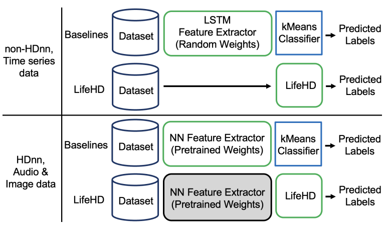
\ Fig. 8 presents a comparison of the pipeline setup using both the baselines and LifeHD on HDnn and non-HDnn frameworks respectively. To ensure fair comparisons, in HDnn framework on ESC-50 and CIFAR-100, we initialize the NN with the same pretrained weights for LifeHD and NN baselines. For the NN baselines on MHEALTH, we randomly initialize a one-layer LSTM of 64 units followed by a fully connected layer of 512 units. This architecture has achieved competitive accuracy as the Transformers-based designs on MHEALTH [12].
\ We compare LifeHD with the following baselines, which include all main lifelong learning techniques:
\ • Finetune is a naïve baseline that optimizes the NN model using the current batch of data without any lifelong learning techniques.
\ • CaSSLe [14] is a distillation-based framework that utilizes self-supervised losses. It leverages distillation between the representations of the current model and a past model. In the original paper, the past model is captured at the end of the previous task and prior to the introduction of a new task.
\

\ However, since we do not assume awareness of task shifts, we simply freeze the model from the previous batch.
\ • LUMP [13] employs a memory buffer for replay and mitigates catastrophic forgetting by interpolating the current batch with previously stored samples in the memory.
\ • STAM [54] is brain-inspired expandable memory architecture using online clustering and novelty detection. We exclusively apply STAM to CIFAR-100 due to its demand for intricate dataset-specific tuning (e.g., number of receptive fields), and because the authors only released the implementation for the CIFAR datasets.
\ • SupHDC [18, 27] is the fully supervised HDC pipeline.
\ All baselines are adapted from their original open-source code. For CaSSLe and LUMP, we employ BYOL [16] as the self-supervised loss function because it has showed superb empirical performance in lifelong learning tasks compared to other self-supervised learning backbones [14]. We use the memory buffer size of 256 for LUMP which is the same as in the original paper. We employ the Stochastic Gradient Descent (SGD) optimizer with a learning rate of 0.03 across all methods, training each batch for 10 steps. All experiments are executed for 3 random trials.
7.4 LifeHD Accuracy
Results on Three Application Scenarios. Fig. 9 (a) details the ACC curve of all methods as streaming samples are received. All NN baselines start at higher accuracy, especially in ESC-50 (sounds) and CIFAR-100 (images), owing to the presence of a pretrained NN feature extractor within the HDnn framework. Meanwhile, LifeHD begins with lower accuracy as both the working and long-term memories are empty, needing to learn the cluster HVs and the optimal number of clusters. Notably, as streaming samples come in,
\

\
![Table 4: The gap of ACCs at the end of the stream between LifeHD and Supervised HDC [18, 27].](https://cdn.hackernoon.com/images/fWZa4tUiBGemnqQfBGgCPf9594N2-8fc302u.png)
\ all NN baselines experience a decline in ACC, underscoring the inherent challenges of unsupervised lifelong learning with streaming non-iid data and a lack of supervision. This is primarily due to the demand for extensive iid data and multi-epoch offline training for finetuning NNs, which is not feasible in our setting. CaSSLe [14] leads to forgetting due to its inability to identify suitable past models from which to distill knowledge. Similarly, LUMP [13] exhibits reduced ACC in ESC-50 and CIFAR-100, with only marginal ACC improvement in MHEALTH (time series), suggesting that its memory interpolation strategy may not be universally suitable for all applications. While the memory-based design of STAM [54] can mitigate forgetting, its efficacy in distinguishing patterns and acquiring new knowledge remains unsatisfactory. On the contrary, LifeHD demonstrates incremental accuracy across all three different scenarios, achieving up to 9.4%, 74.8% and 11.8% accuracy increase on MHEALTH (time series), ESC-50 (sound) and CIFAR100 (images), compared with the NN-based unsupervised lifelong learning baselines at the end. Such outcome can be attributed to HDC’s lightweight but meaningful encoding and the effective memorization design of LifeHD.
\ Results under Data Distribution Drift. We further evaluate LifeHD’s performance under drifted data and present the final ACC along with the number of discarded cluster HVs in Fig. 9 (b). Specifically, we introduce gradual rotation to the CIFAR-100 samples within each class, ranging from no rotation to a substantial rotation angle of 80◦ . The other parameter settings remain the same as in Table 3. The number of discarded cluster HVs accounts for those that are either forgotten or merged. From Fig. 9 (b), we can observe the remarkable resilience of LifeHD to drifted data, with an ACC loss of less than 2.3% even under a severe rotation of 80◦ . This robustness stems from the general and uniform design of LifeHD to accommodate various types of continuously changing data streams. In cases of slight or minimal distribution drift, LifeHD updates existing cluster HVs; in instances of severe drift, new cluster HVs are created and subsequently merged if deemed appropriate. However, due to the finite memory capacities, more cluster HVs are subject to forgetting or merging under larger drifts, as shown in Fig. 9 (b) by the number of discarded cluster HVs, leading to ACC
\

\ loss. In our experiments, LifeHD demonstrates minimal ACC loss even under substantial rotation shifts.
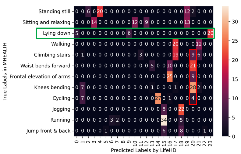
\ Comparison with Fully Supervised HDC. Table 4 compares the average ACCs of supervised HDC method [18, 27] and LifeHD. Even without any supervision, LifeHD approaches the ACC of supervised HDC with a gap of 15%, 3% and 6% on MHEALTH, ESC-50 and CIFAR-100. A minimal ACC gap confirms the effectiveness of LifeHD in separating and memorizing key patterns. To help explain the small ACC loss even without supervision, we visualize the confusion matrix of LifeHD on MHEALTH in Fig. 10. MHEALTH has 12 true classes (y axis), whereas LifeHD maintains 23 cluster HVs in its long-term memory (x axis). ACC is evaluated by mapping the unsupervised cluster HVs to true labels. Although LifeHD cannot achieve precise label matching with true classes, it can preserve the essential patterns by using finer-grained clusters. For example, the green box in Fig. 10 highlights a valid learning outcome, where LifeHD uses predicted cluster HV No. 0, 9 and 23 to represent a bigger true class of “Lying down”.
7.5 Training Latency and Energy
Fig. 11 provides comprehensive latency and energy consumption results to train one batch of samples on all three edge platforms. For CIFAR-100, we use the most lightweight MobileNet version, V3 small [20], as HDnn feature extractor and NN baseline, to assess LifeHD’s efficiency gain over the most competitive mobile computing setup. On RPi Zero, we report results for the relatively lightweight NN-based baselines, Finetune and LUMP [13], using
\

\

\ the smallest dataset, MHEALTH, while running CaSSLe [14] on MHEALTH would result in out-of-memory errors. As shown in Fig. 11, LifeHD is up to 23.7x, 36.5x and 22.1x faster to train on RPi Zero, RPi 4B and Jetson TX2, respectively, while being up to 22.5x, 34.3x and 20.8x more energy efficient on each, compared to the NN-based unsupervised lifelong learning baselines. In most settings, CaSSLe [14] is the most time-consuming because of the expensive distillation. LUMP [13] is slightly more expensive than Finetune due to its replay mechanism. STAM [54], implemented only on CPU, incurs the longest training latency on Jetson TX2, as it does not use GPU’s acceleration capabilities. LifeHD is clearly faster and more efficient than all NN-based unsupervised lifelong learning baselines [13, 14, 54] due to LifeHD’s lightweight nature. The overhead of LifeHD alongside fully supervised HDC, SupHDC [18, 27], is negligible on more powerful platforms like RPi 4B and Jetson TX2. Notably, in LifeHD, the cluster HV merging step for processing about 40 LTM elements takes 7.4, 0.86 and 0.66 seconds to run on RPi Zero, RPi 4B and Jetson TX2, respectively, which only executes once every 𝑓𝑚𝑒𝑟𝑔𝑒 batches. Further enhancements can be achieved using the acceleration techniques mentioned in Sec. 5.4.
\ Fig. 11 indicates LifeHD improves latency and energy efficiency the most on RPi 4B, as compared to RPi Zero and Jetson TX2 that represent more limited or powerful devices. This is because the highdimensional nature of LifeHD requires a fair amount of memory, thus it cannot run efficiently on the highly restricted RPi Zero. The GPU resources on Jetson TX2 boost the NN-based baselines, narrowing the gap between them and LifeHD. We expect much larger efficiency improvements when LifeHD is accelerated using emerging in-memory computing hardware [11, 65].
7.6 Memory Usage
Fig. 12 provides a comprehensive summary of peak memory footprint for all methods on MHEALTH and CIFAR-100. We categorize the methods into NN training (Finetune, LUMP [13], CaSSLe [14], STAM [54]) and HDC training (Supervised HDC [18, 27] and our LifeHD). Following [30], we calculate the peak memory of NN training as the sum of model, optimizer and activation memories, plus additional memory consumption for lifelong learning. Specifically, CaSSLe [14] requires additional memory for training a predictor and inference from a frozen model, LUMP [13] needs extra memory for replay. For HDC-based methods, each dimension of the cluster HV is represented as a signed integer and stored in a byte. In addition to the working and long-term memories, we also consider the storage of bipolar level and ID hypervectors for encoding, and the frozen MobileNet for HDnn encoding in CIFAR-100. Notice that our focus here is on comparing full-precision memory usage, and optimization techniques like quantization can be applied to all methods in the future.
\ The results in Fig. 12 highlight LifeHD’s memory efficiency. LifeHD conserves 80.1%-86.2% and 84.1%-96.0% of memory compared to NN training baselines on MHEALTH (non-HDnn) and CIFAR-100 (HDnn), respectively. This remarkable efficiency stems from LifeHD’s HDC design, which dispenses with the memoryintensive gradient descents in NNs. STAM [54], with its hierarchical and expandable memory structure, consumes 6.3x the memory of LifeHD, as it stores raw image patches across all hierarchies. Compared to fully supervised HDC, SupHDC [18, 27], LifeHD introduces a modest memory increase to accomplish the challenging task of organizing label-free cluster HVs. LifeHD proves advantageous for edge applications with only 103 KB and 2.5 MB of peak memory required for MHEALTH and CIFAR-100.
7.7 Ablation Studies
The design of LifeHD consists of several key elements: the two-tier memory organization, novelty detection and online update, and cluster HV merging that manipulates past patterns. We conduct experiments to assess the contribution of each element. Using the configuration in Table 3, we evaluate the performance of (i) LifeHD without long-term memory, using only a single layer memory, (ii) LifeHD without merging, employing only novelty detection, online update and forgetting, and (iii) complete LifeHD. We present the ACC and the number of cluster HVs in LTM during MHEALTH training in Fig. 13, chosen as a representative scenario. LifeHD without LTM (green dashdot line) forces cluster HV merging to
\

\ take place in working memory, where the large number of temporary cluster HVs creates less important nodes in the graph and corrupts the graph-based merging process, as shown in Fig. 13 (left). This necessitates the design of the two-tier memory architecture and merging with LTM elements. LifeHD without merging (blue dashed line) consumes 1x more memory in the LTM, making it unsuitable for resource-constrained edge devices. Our design of LifeHD (red solid line) strategically combines similar cluster HVs with minor loss on the clustering quality, achieving ACC similar to those without merging while conserving memory storage.
7.8 Sensitivity Analysis
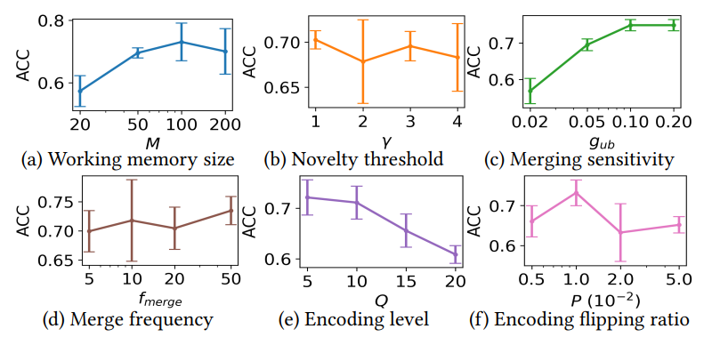
Fig. 14 summarizes the sensivitity results of key parameters in LifeHD, while the less sensitive ones such as 𝛼 and ℎ𝑖𝑡𝑡ℎ are omitted due to space limitation. The default setting is the same as in Table 3.
\ Working Memory Size. Fig. 14 (a) shows ACCs using working memory sizes of 20, 50, 100 and 200. In general, a larger working memory allows more temporary cluster HVs at the cost of higher memory consumption. 𝑀 = 100 produces optimal results, while further increasing the memory size reduces clustering quality. This occurs because excessively large working memory retains outdated prototypes, degrading lifelong learning performance.
\ Novelty Threshold. In Fig. 14 (b), we present the final ACCs for different novelty detection thresholds (𝛾). A lower 𝛾 results in more frequent novelty detections and increased loads on the working memory, while a higher 𝛾 may lead to overlooking significant changes. Remarkably, LifeHD demonstrates resilience to variations in 𝛾, a phenomenon that we attribute to the combined impact of novelty detection and merging processes.
\ Merging Sensitivity. Fig. 14 (c) shows ACC using various merging thresholds (𝑔𝑢𝑏). 𝑔𝑢𝑏 determines the number of clusters (𝑘) to merge in the cluster HV merging step (Sec. 5.4). A low value for 𝑔𝑢𝑏 results in overly aggressive merging, leading to the fusion of dissimilar cluster HVs and a degraded ACC. A larger 𝑔𝑢𝑏 adopts a conservative merging strategy and encourages finer-grained clusters, albeit at the expense of increased resource demands.
\ Merging Frequency. Fig. 14 (d) shows the final ACCs for different merging frequencies (𝑓𝑏𝑎𝑡𝑐ℎ). LifeHD shows its robustness across various 𝑓𝑏𝑎𝑡𝑐ℎ values, partly due to the presence of 𝑔𝑢𝑏 to prevent aggressive merging. Less frequent merging (larger 𝑓𝑏𝑎𝑡𝑐ℎ) raises the risk of forgetting important patterns as of memory constraints. More frequent merging (smaller 𝑓𝑏𝑎𝑡𝑐ℎ) increases the computational burden due to the spectral clustering-based algorithm.
\ Encoding Level and Flipping Ratio for Spatiotemporal Encoding. Fig. 14 (e) and (f) show the ACCs for various quantization encoding levels (𝑄) and flipping ratios (𝑃) during the spatiotemporal encoding. Both parameters are important for preserving the
\

\ similarity in HD-space after encoding. Optimal 𝑄 depends on the sensor sensitivity, with finer-grained sensors requiring more quantization levels. 𝑃 determines the similarity between adjacent levels of hypervectors. For personal health monitoring, such as MHEALTH, 𝑄 = 10, 𝑃 = 0.01 usually gives the best results.
\
:::info This paper is available on arxiv under CC BY-NC-SA 4.0 DEED license.
:::
\
This content originally appeared on HackerNoon and was authored by Computational Technology for All
Computational Technology for All | Sciencx (2024-07-24T18:00:20+00:00) Lifelong Intelligence Beyond the Edge using Hyperdimensional Computing: Evaluation of LifeHD. Retrieved from https://www.scien.cx/2024/07/24/lifelong-intelligence-beyond-the-edge-using-hyperdimensional-computing-evaluation-of-lifehd/
Please log in to upload a file.
There are no updates yet.
Click the Upload button above to add an update.
