This content originally appeared on HackerNoon and was authored by Kashintsev Georgii
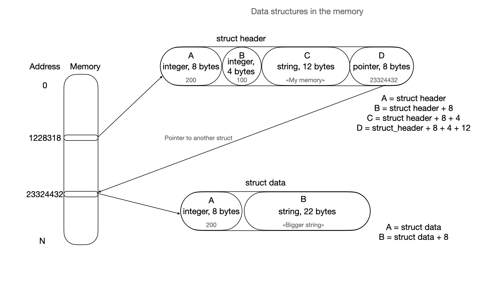
Data structures are a serious tool to store data conveniently. Memory in machines is a sequential space, which can be addressed from 0 to N. Managing this space is difficult, but it discovers possibilities of storing data in computer systems as a routine operation and it qualitatively distinguishes well-organized memory working software from others. It also makes it possible to put chaotic data in order.
\ In common, data structures use only two addressing methods:
- pointer to address
- offset from pointer
\ Simply any data in the memory can be represented as:
\ Array can be represented like this:
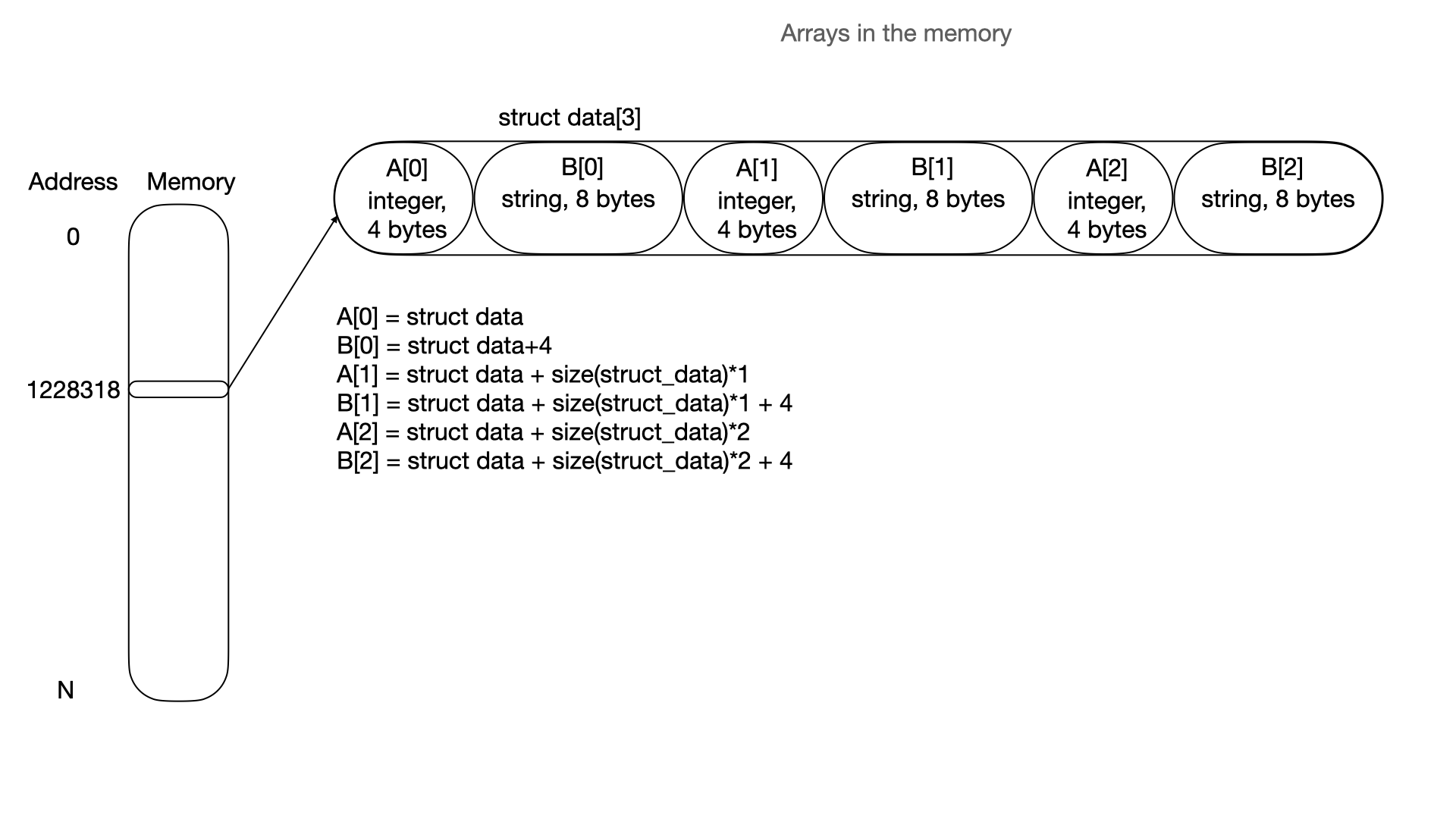
\ All ideas are based on this logic. If an application uses a pointer to pointer addressing method - this is linked-list mechanics. A linked list and trees use a lot of pointer to pointer mechanics, whereas hash tables, bitmaps and heaps are using arrays (basically, this is a pointer + offset addressing method to each element).
Key-Value associative arrays (or maps)
The most popular data structure for this is a hash table. Sometimes it can be made with RB or B-tree.
\ Hash tables are popular due to the ability of fast access to any element - O(1). O(1) in big-O notation means the constant time taken to access every element. O(1) might seem an unclear way to express access time, but the main thing is that access time doesn’t depend on the amount of elements in a hash table. It’s not an absolute value and it cannot be converted to time measures. This is a way to compare how much size of data structures influences time characteristics of operations processed with a data structure. O(1) converted in time spent on an operation with a data structure will be different from O(1) in another data structure.
\
Two quite efficient dependencies in big-O notation are constant (O(1)) and logarithm (O(ln(n), where “n” is the amount of elements stored in data structure). They have optimal access time to any element in comparison to linear dependency. The main idea of this - absence of significant increasing access time while data structure is filling. \n 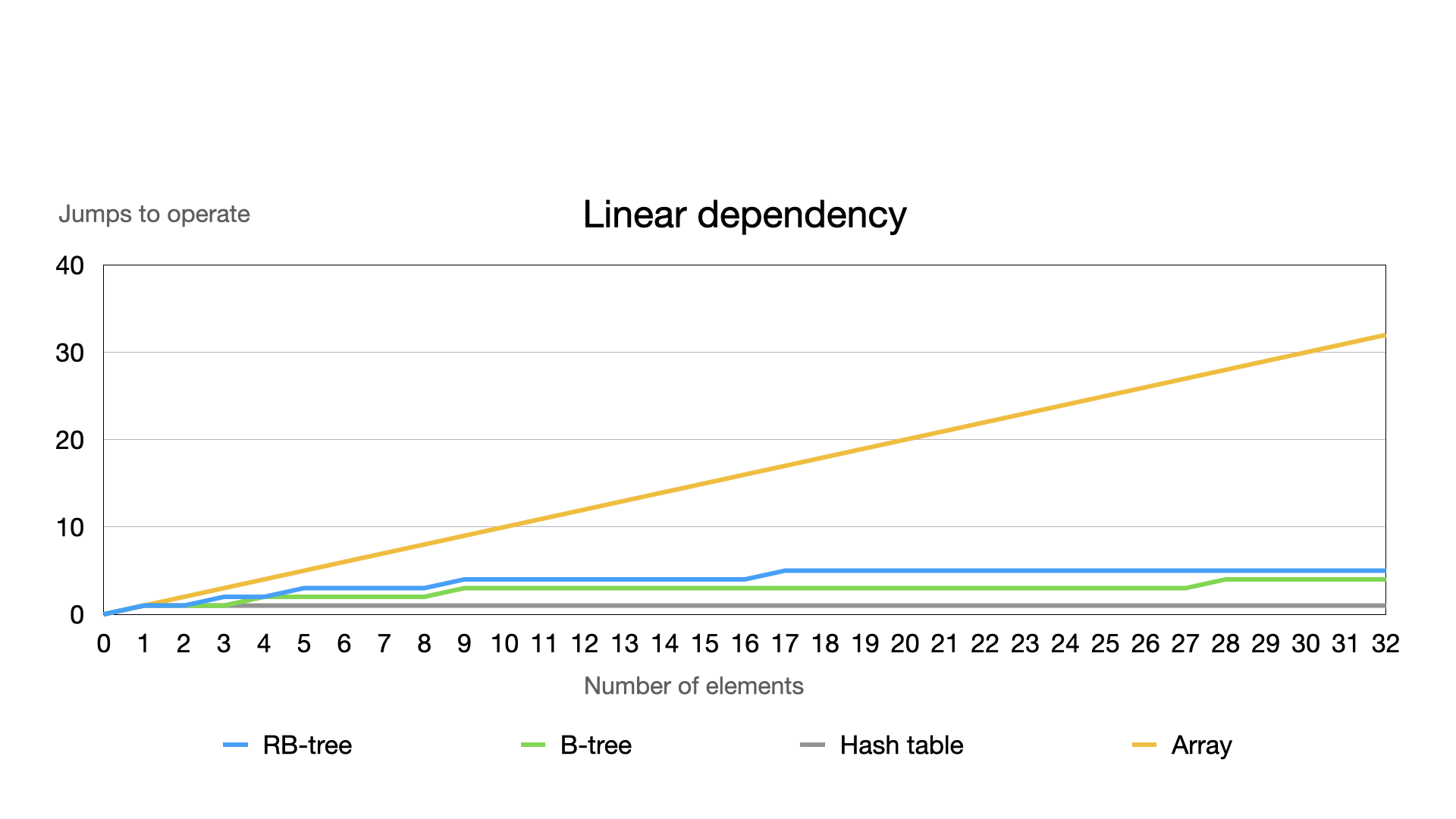
\ The chart above considers a small range of numbers of elements. If we expand this, the array will increase too fast. Then, let’s see the difference by recreating this graph, using a logarithm scale excluding arrays as they are not efficient.
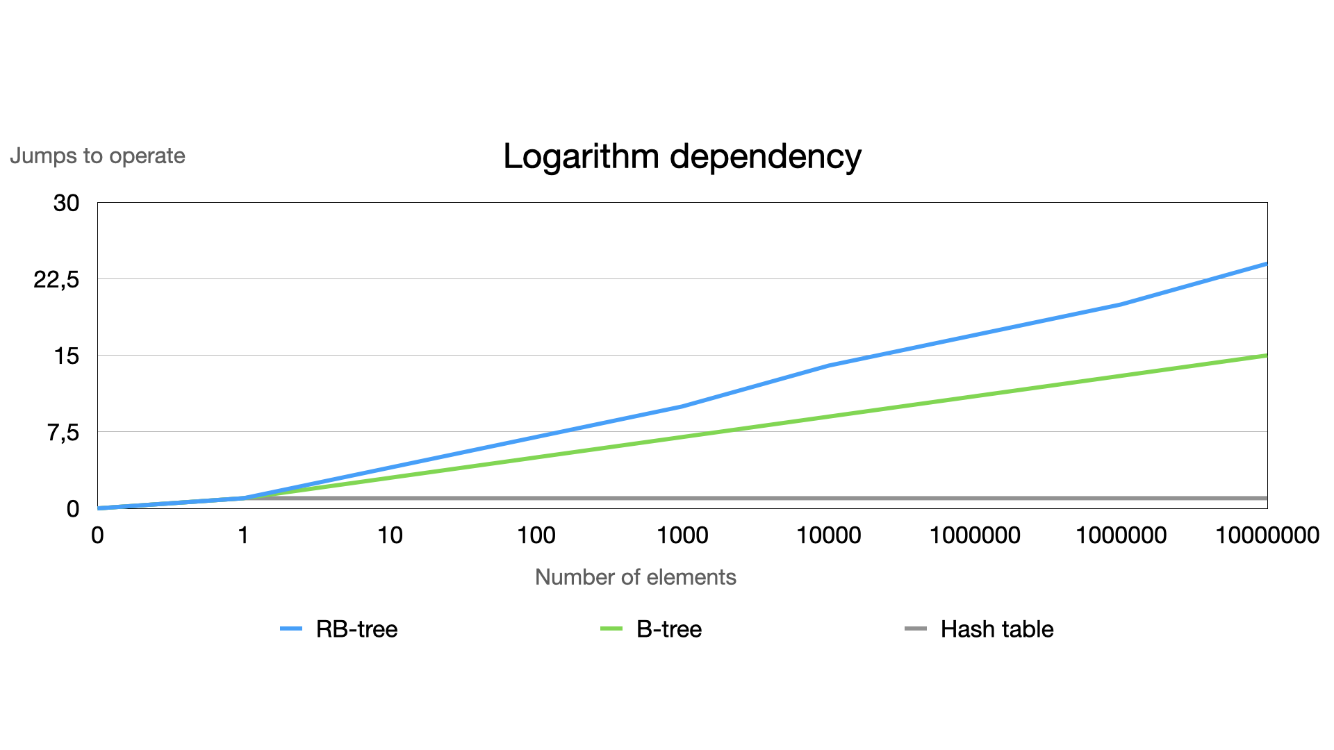 In most cases, a hash table is sufficient. However, hash tables have problems with resize and sometimes it’s time-consuming to add new elements as some insertions require recreating the array for data of the hash table.
\ In turn, trees have their own set of advantages. Various types of trees make applications more flexible because they can do the selection. Inexact search is the main task for using trees. It can look for near objects (as in geospatial K-D or R-tree), objects with index less than N (in B or RB-tree), keys with prefix or suffix (as in radix tree), most recently used objects in splay tree and so on.
\n Efficient sorting by the tree
There are many sorting algorithms based on an array with high computational complexity. All sorting algorithms have linearly dependent complexity.
\ On the other hand, applications with Heap or with an RB-tree order data by default (but without an indexed method to access).
\ RB-tree is an ordered tree, which is classified as a Binary Search Tree. Every node of the tree has a key. All keys are ordered from left to the right, ascending or descending. Binary trees must have the comparing function. These functions can route keys with data through the tree. The compare function must prepare the answer: store or find the current key on the left or right branch.
\ A format of the key can be different: it can be integer, string or even struct with some amount of keys. In each of these cases the compare function must always know the answer where to look for or put: in the right or left branch.
\ Let’s consider an example. To simplify, I’ve reduced the code to pure Binary Tree, removing fixup rotations and other complexities like “deletion” mechanics. These are really complicated functions with a lot of tree balancing logic. Binary trees are always ordered and these functions don’t matter in our case.
\
#include <stdlib.h>
#include <string.h>
#include <stdio.h>
#define BLACK 1
#define RED 2


typedef struct node_t {
    struct node_t *left;
    struct node_t *right;
    int color;

    char *key;
    char *data;
} node_t;

typedef struct tree_t {
    node_t *root;
    int count;
} tree_t;

node_t* node_make(char *key, char *data, int color) {
    node_t *node = calloc(1, sizeof(*node));
    node->key = strdup(key);
    node->data = strdup(data);
    node->color = color;

    return node;
}

int cmp_function(char *one, char *another) {
    return strcmp(one, another);
}

node_t *tree_insert(tree_t *tree, char *key, char *value) {
    node_t *node = tree->root;
    if (!node) {
        tree->root = node_make(key, value, BLACK);
        ++tree->count;
    }


    while (node) {
        int rc = cmp_function(node->key, key);
        if (rc > 0)
            if (node->left)
                node = node->left;
            else
            {
                node->left = node_make(key, value, RED);
                ++tree->count;
                return node->left;
            }
        else if (rc < 0)
            if (node->right)
                node = node->right;
            else
            {
                node->right = node_make(key, value, RED);
                ++tree->count;
                return node->right;
            }
        else {
            return NULL;
        }
    }

    return NULL;
}

node_t* tree_get(tree_t *tree, char *key) {
    node_t *node = tree->root;
    while (node) {
        int rc = cmp_function(node->key, key);
        if (rc > 0)
            node = node->left;
        else if (rc < 0)
            node = node->right;
        else
            return node;
    }

    return NULL;
}

void node_callback(node_t *node, void (*callback)(node_t*, void*), void *arg) {
    if (!node)
        return;

    node_callback(node->left, callback, arg);
    callback(node, arg);
    node_callback(node->right, callback, arg);
}

void tree_foreach(tree_t *tree, void (*callback)(node_t*, void*), void *arg) {
    node_callback(tree->root, callback, arg);
}

void print_node(node_t *node, void* arg) {
    printf("node->key='%s', node->data='%s'\n", node->key, node->data);
}

int main() {
    tree_t *tree = calloc(1, sizeof(*tree));

    tree_insert(tree, "Casablanca", "Morocco");
    tree_insert(tree, "Delhi", "India");
    tree_insert(tree, "Istanbul", "Turkey");
    tree_insert(tree, "Osaka", "Japan");
    tree_insert(tree, "Prague", "Czech Republic");
    tree_insert(tree, "Sydney", "Australia");
    tree_insert(tree, "Tashkent", "Uzbekistan");
    tree_insert(tree, "Valencia", "Venezuela");
    tree_insert(tree, "Kyoto", "Japan");
    tree_insert(tree, "Hamburg", "Germany");
    tree_insert(tree, "Warsaw", "Poland");
    tree_insert(tree, "Berlin", "Germany");
    tree_insert(tree, "Yokohama", "Japan");
    tree_insert(tree, "Zhengzhou", "China");
    tree_insert(tree, "Ankara", "Turkey");
    node_t *node_get = tree_get(tree, "Ankara");
    if (node_get)
        printf("node key val: '%s'\n", node_get->data);

    tree_foreach(tree, print_node, NULL);
}
\ Firstly, take a look at the compare function. It is just a call to another function called “strcmp”. This function compares letters in two strings from the beginning to the end. If a letter in one word is greater than a letter in the second word in the same position (alphabetically greater, for example, b > a), the function returns 1. If it is less than the letter in the second word, then return -1. If two words are equal, then the function returns 0. It discovers application opportunities to compare words. In the Binary Tree logic, it also guarantees that get and insert functions use the similar routing to find or insert elements. Compare function controls the routing through the tree.
\ As a result, let’s try to run it:
node->key='Ankara', node->data='Turkey'
node->key='Berlin', node->data='Germany'
node->key='Casablanca', node->data='Morocco'
node->key='Delhi', node->data='India'
node->key='Hamburg', node->data='Germany'
node->key='Istanbul', node->data='Turkey'
node->key='Kyoto', node->data='Japan'
node->key='Osaka', node->data='Japan'
node->key='Prague', node->data='Czech Republic'
node->key='Sydney', node->data='Australia'
node->key='Tashkent', node->data='Uzbekistan'
node->key='Valencia', node->data='Venezuela'
node->key='Warsaw', node->data='Poland'
node->key='Yokohama', node->data='Japan'
node->key='Zhengzhou', node->data='China'
\ This is an efficient code which requires only a small number of operations to insert or retrieve elements. Inserting or retrieving an element takes only 20 steps through the tree. In contrast, an application with an array process must check all elements.
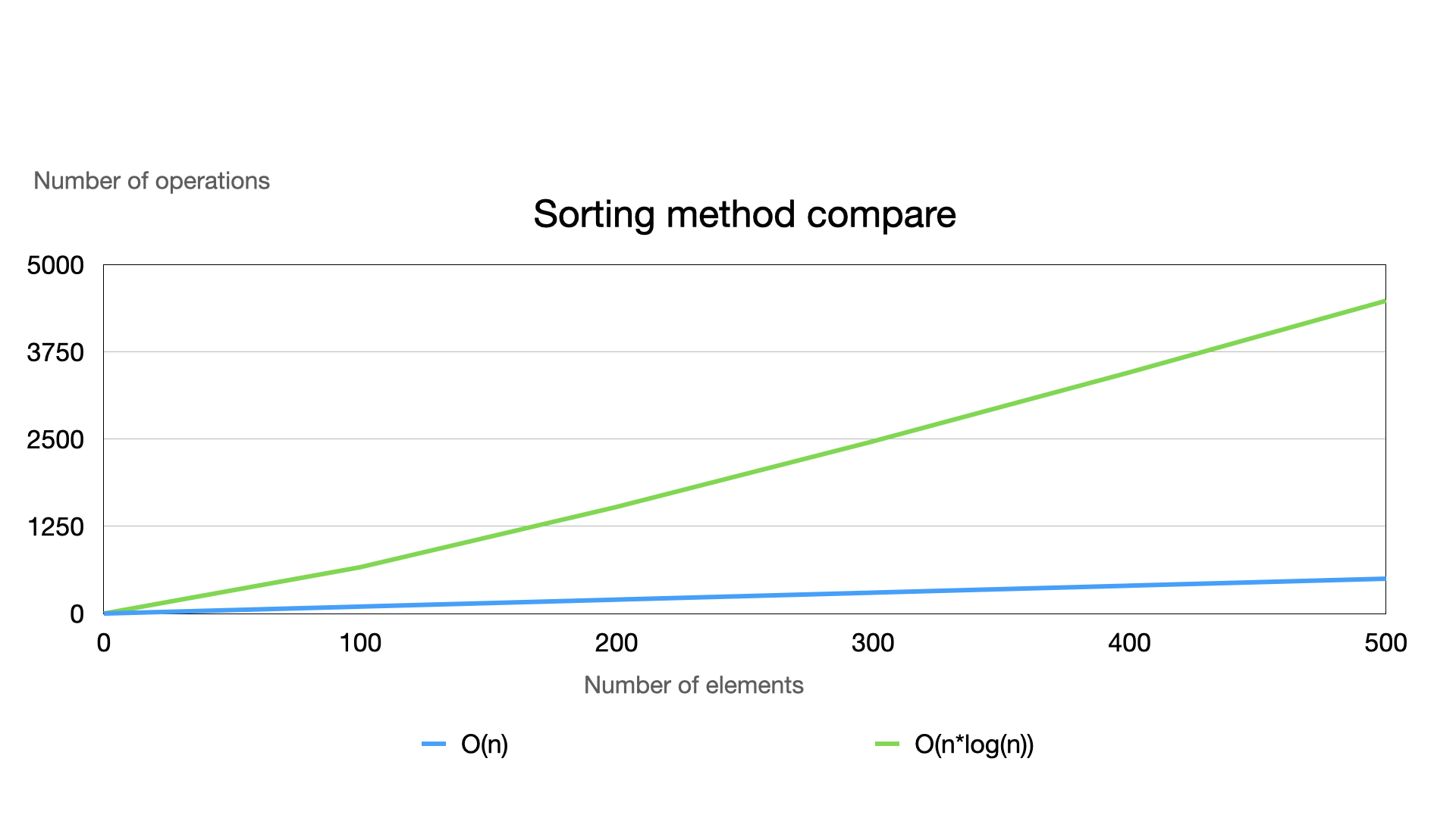
\ What about sorting? Let's try to compare RB trees with sorting algorithms. There are two most efficient algorithms: quick sort and heap sort. Their sorting time is compared by the formula: O(n*log(n)).
\ In a binary tree there’s only scanning time of a tree, i.e. O(n), because the tree is already sorted by default.
\
\ Sometimes applications need to work with array data. For instance, it should be possible to calculate the quantiles using indexes to access elements. In such cases, callback functions can be changed from print to filling the array. To simplify the code we can direct the second argument to callback function: \n
void node_callback(node_t *node, void (*callback)(node_t*, void*, void*), void *arg, void *arg2) {
    if (!node)
        return;

    node_callback(node->left, callback, arg, arg2);
    callback(node, arg, arg2);
    node_callback(node->right, callback, arg, arg2);
}

void tree_foreach(tree_t *tree, void (*callback)(node_t*, void*, void*), void *arg, void *arg2) {
    node_callback(tree->root, callback, arg, arg2);
}
\ and then, use it in the main function:
    int size = tree_size(tree);
    char *arr[size];
    int i = 0;
    tree_foreach(tree, make_array, arr, &i);
    for (i = 0; i < size; ++i) {
        printf("%s\n", arr[i]);
    }
\ This callback function creates a sorted array, after which the application prints the results to the screen:
Ankara
Berlin
Casablanca
Delhi
Hamburg
Istanbul
Kyoto
Osaka
Prague
Sydney
Tashkent
Valencia
Warsaw
Yokohama
Zhengzhou
\
Multi-dimensional or multi-key data structures
When it is necessary to have a map with two keys, the solution is to make a map of a map (or dictionaries of dictionaries, depending on the programming language). However, this approach may not be very efficient as it involves performing two searches. Moreover, in languages without automatic memory management it causes more challenges as instead of one struct with manual memory management, the application has a lot of other data structures, which are linked to the keys of the first.
\ Another approach involves combining keys in string format. Here’s the example of a code below when it is necessary to insert and search for cities within countries. Different countries have cities with similar names. Hence, we will use a connected key format: “country:city”. For example, these keys look like “Japan:Tokyo”. This is an efficient way because the application should iterate over only one data structure.
\ The third approach involves using multikey data structures. In the RB tree it is enabled through comparison functions and the possibility of adding the second (or more) keys:
\
node_t *tree_insert(tree_t *tree, char *city_key, char *country_key, int value);
node_t* tree_get(tree_t *tree, char *city_key, char *country_key);

int cmp_function(char *city_expect, char *city_key, char *country_expect, char *country_key) {
    int rc;

    if ((rc = strcmp(city_key, city_expect)))
        return rc;

    if ((rc = strcmp(country_key, country_expect)))
        return rc;

    return 0;
}
\ To simplify, let’s alter the data type of value to integer, because in this case it doesn’t matter.
\ Let’s rewrite the code in the main function like this:
    tree_insert(tree, "Cairo", "USA", 1);
    tree_insert(tree, "Sydney", "Canada", 2);
    tree_insert(tree, "Istanbul", "Turkey", 3);
    tree_insert(tree, "Osaka", "Japan", 4);
    tree_insert(tree, "Waterloo", "Belgium", 5);
    tree_insert(tree, "Sydney", "Australia", 6);
    tree_insert(tree, "Tashkent", "Uzbekistan", 7);
    tree_insert(tree, "Waterloo", "Canada", 8);
    tree_insert(tree, "Kyoto", "Japan", 9);
    tree_insert(tree, "Hamburg", "Germany", 10);
    tree_insert(tree, "Warsaw", "Poland", 11);
    tree_insert(tree, "Berlin", "Germany", 12);
    tree_insert(tree, "Yokohama", "Japan", 13);
    tree_insert(tree, "Zhengzhou", "China", 14);
    tree_insert(tree, "Ankara", "Turkey", 15);
    tree_insert(tree, "Cairo", "Egypt", 16);
    node_t *node_get = tree_get(tree, "Sydney", "Canada");
    if (node_get)
        printf("node key val: '%d'\n", node_get->data);

    tree_foreach(tree, print_node, NULL, NULL);
\ These insert and get functions work with two keys. The rest of the code isn’t distinguished so far, only the number of arguments are changed. In this code, if names of cities are unique, then data structure works as a one-dimensional tree. When city names are found two or more times, the tree sorts them by a city name and then by a country name. The Application displays these results on the console:
node key val: '2'
country='Turkey', city='Ankara'
country='Germany', city='Berlin'
country='Egypt', city='Cairo'
country='USA', city='Cairo'
country='Germany', city='Hamburg'
country='Turkey', city='Istanbul'
country='Japan', city='Kyoto'
country='Japan', city='Osaka'
country='Australia', city='Sydney'
country='Canada', city='Sydney'
country='Uzbekistan', city='Tashkent'
country='Poland', city='Warsaw'
country='Belgium', city='Waterloo'
country='Canada', city='Waterloo'
country='Japan', city='Yokohama'
country='China', city='Zhengzhou'
\
Expire mechanics
Expire mechanics (deleting old data) is a common task in database management. Some amount of data can be stored in KV-databases with expiration times. It forces the database to delete old keys which are not actual.
\ For example, Redis database uses different approaches:
- passive key expiration (expires when user requests the element)
- random sampling to delete expired keys (it reduces CPU load in comparison with a full scan)
- The radix tree was implemented to reduce the amount of sampling data in version 6
As another example, nginx uses RB-tree quite extensively:
- To expire old events in eventloop
- Here’s an interesting method: an RB tree with the option to specify a custom insert function. In this example you can see how to customize not only the compare function, but also the insert process
\ In the Linux kernel the RB tree is used in the CFS CPU scheduler to compare the CPU time of processes with small CPU usage to arrange the priority. This task is similar to an expiration handling as the scheduler needs to identify the ordered process with the minimal CPU usage.
\ Besides, trees are useful for imprecise operations. They can be found in all keys which have a key lesser or greater than searching.
\ The next code example will be similar to the previous one, based on Binary trees. However, in this case, we can't limit ourselves by using a simple Binary tree due to the need for deletion functions. Another reason for using RB tree mechanics - using sequential increasing keys while elements are added. As a result, this leads to significant imbalance in the tree, essentially transforming it into a Linked list.
\ Red-Black (RB) trees are the only extension of the common Binary Tree. All nodes in the RB tree have a color. New nodes are initially colored red. If the tree contains at least a red parent which is connected to the red child then the tree is imbalanced. The balancing mechanics are not covered in this article. The internet has enough information about this. Only two remarks - the functions left and right rotate transfer elements between different branches. During insertions or deletions, the tree may undergo a fixup to rearrange nodes through the tree from the operating node to the root. Then, some insertions or deletions may have complexity of approximately 2*log2(n).
\ To make an opportunity to find a parent, add the pointer ‘parent’ to the node and to the function called node_make. It ensures that all nodes (except a root) have a parent.However, this code has a clear problem: it doesn’t free up the memory from the node after deletion as the foreach mechanics might simultaneously use this node. Implementation of Garbage Collection can be a solution for this. As another way, old elements could be placed in the buffer (such as a Linked List) and it’s necessary to scan this buffer to free the memory after.
\ The common structs and code are updated:
\
#include <stdlib.h>
#include <string.h>
#include <stdio.h>
#define BLACK 1
#define RED 2

typedef struct node_t {
    struct node_t *left;
    struct node_t *right;
    struct node_t *parent;
    int color;

    int key;
    char* data;
} node_t;

typedef struct tree_t {
    node_t *root;
    int count;
} tree_t;

node_t* node_make(int key, char* data, int color, node_t *parent) {
    node_t *node = calloc(1, sizeof(*node));
    node->key = key;
    node->data = strdup(data);
    node->color = color;
    node->parent = parent;

    return node;
}

int cmp_function(int expect, int key) {
    int rc;

    if (key > expect)
        return 1;

    if (key < expect)
        return -1;

    return 0;
}

void left_rotate(tree_t *tree, node_t *node) {
    node_t *branch = node->right;
    node->right = branch->left;
    if (branch->left) {
        branch->left->parent = node;
    }
    branch->parent = node->parent;
    if (!node->parent) {
        tree->root = branch;
    }
    else if (node == node->parent->left) {
        node->parent->left = branch;
    }
    else {
        node->parent->right = branch;
    }
    branch->left = node;
    node->parent = branch;
}

void right_rotate(tree_t *tree, node_t *node) {
    node_t *branch = node->left;
    node->left = branch->right;
    if (branch->right) {
        branch->right->parent = node;
    }
    branch->parent = node->parent;
    if (!node->parent) {
        tree->root = branch;
    }
    else if (node == node->parent->right) {
        node->parent->right = branch;
    }
    else {
        node->parent->left = branch;
    }
    branch->right = node;
    node->parent = branch;
}
\ Here is the insertion code below. It has a fixup function which conducts the tree from the new node to the root and checks sequentially connected two and more nodes marked as RED. It performs rotations over the branches and changes the color of the nodes to black.
\
void insertion_fixup(tree_t *tree, node_t *node) {
    if (!node || !node->parent)
        return;

    while(node->parent->color == RED) {
        if(node->parent == node->parent->parent->left) {

            node_t *gp_branch = node->parent->parent->right;

            if(gp_branch && gp_branch->color == RED) {
                node->parent->color = BLACK;
                gp_branch->color = BLACK;
                node->parent->parent->color = RED;
                node = node->parent->parent;
            }
            else {
                if(node == node->parent->right) {
                    node = node->parent;
                    left_rotate(tree, node);
                }
                node->parent->color = BLACK;
                node->parent->parent->color = RED;
                right_rotate(tree, node->parent->parent);
            }
        }
        else {
            node_t *gp_branch = node->parent->parent->left;

            if(gp_branch && gp_branch->color == RED) {
                node->parent->color = BLACK;
                gp_branch->color = BLACK;
                node->parent->parent->color = RED;
                node = node->parent->parent;
            }
            else {
                if(node == node->parent->left) {
                    node = node->parent;
                    right_rotate(tree, node);
                }
                node->parent->color = BLACK;
                node->parent->parent->color = RED;
                left_rotate(tree, node->parent->parent);
            }
        }

        if (!node->parent)
            break;
    }
    tree->root->color = BLACK;
}

node_t *tree_insert(tree_t *tree, int key, void* value) {
    node_t *node = tree->root;
    node_t *new = NULL;
    if (!node)
    {
        tree->root = new = node_make(key, value, BLACK, NULL);
        ++tree->count;
    }

    while (node) {
        int rc = cmp_function(node->key, key);
        if (rc > 0)
            if (node->right)
                node = node->right;
            else
            {
                node->right = new = node_make(key, value, RED, node);
                ++tree->count;
                insertion_fixup(tree, new);
                return new;
            }
        else if (rc < 0)
            if (node->left)
                node = node->left;
            else
            {
                node->left = new = node_make(key, value, RED, node);
                insertion_fixup(tree, new);
                ++tree->count;
                return new;
            }
        else {
            return NULL;
        }
    }

    return new;
}
\ Here is the delete function below. It has much fixup logic and much complex deletion mechanics.
void rb_delete_fixup(tree_t *tree, node_t *node) {
    while(node && node != tree->root && node->color == BLACK) {
        if (!node->parent)
            break;

        if(node == node->parent->left) {
            node_t *p_branch = node->parent->right;
            if (!p_branch)
                break;

            if(p_branch->color == RED) {
                p_branch->color = BLACK;
                node->parent->color = RED;
                left_rotate(tree, node->parent);
                p_branch = node->parent->right;
            }
            if(p_branch->left && p_branch->left->color == BLACK && p_branch->right && p_branch->right->color == BLACK) {
                p_branch->color = RED;
                node = node->parent;
            }
            else {
                if(p_branch->left && p_branch->right->color == BLACK) {
                    p_branch->left->color = BLACK;
                    p_branch->color = RED;
                    right_rotate(tree, p_branch);
                    p_branch = node->parent->right;
                }
                if (!p_branch->left)
                    break;

                p_branch->color = node->parent->color;
                node->parent->color = BLACK;
                p_branch->right->color = BLACK;
                left_rotate(tree, node->parent);
                node = tree->root;
            }
        }
        else {
            node_t *p_branch = node->parent->left;
            if (!p_branch)
                break;

            if(p_branch->color == RED) {
                p_branch->color = BLACK;
                node->parent->color = RED;
                right_rotate(tree, node->parent);
                p_branch = node->parent->left;
            }
            if(p_branch->right && p_branch->right->color == BLACK && p_branch->left && p_branch->left->color == BLACK) {
                p_branch->color = RED;
                node = node->parent;
            }
            else {
                if(p_branch->left && p_branch->right && p_branch->left->color == BLACK) {
                    p_branch->right->color = BLACK;
                    p_branch->color = RED;
                    left_rotate(tree, p_branch);
                    p_branch = node->parent->left;
                }
                if (!p_branch->left)
                    break;

                p_branch->color = node->parent->color;
                node->parent->color = BLACK;
                p_branch->left->color = BLACK;
                right_rotate(tree, node->parent);
                node = tree->root;
            }
        }
    }

    if (node)
        node->color = BLACK;
}


node_t* rb_transfer(tree_t *tree, node_t *node, node_t *branch) {
    if (!node->parent)
        tree->root = branch;
    else if (node == node->parent->left) {
        node->parent->left = branch;
    }
    else if (node == node->parent->right) {
        node->parent->right = branch;
    }

    if (branch) {
        branch->parent = node->parent;
    }

    return node;
}

node_t* minimum(node_t *node) {
    while (node && node->left)
        node = node->left;
    return node;
}

node_t* rb_delete(tree_t *tree, node_t *node) {
    if (!node)
        return NULL;

    node_t *y = node;
    node_t *x;
    int y_orignal_color = y->color;
    node_t* ret = node;

    if (!node->left) {
        x = node->right;
        ret = rb_transfer(tree, node, x);
    }
    else if (!node->right) {
        x = node->left;
        ret = rb_transfer(tree, node, x);
    }
    else {
        y = minimum(node->right);
        y_orignal_color = y->color;
        x = y->right;

        if (y->parent == node) {
            ret = rb_transfer(tree, node, y);
            y->left = node->left;
            node->left->parent = y;
        } else {
            node_t *y_parent = y->parent;
            y_parent->left = x;

            if (x)
            {
                x->parent = y_parent;
            }

            y->right = node->right;

            ret = rb_transfer(tree, node, y);
            y->left = node->left;
            y->right = node->right;
            y->parent = node->parent;
            node->left->parent = y;
            node->right->parent = y;

            y->color = node->color;
        }
    }

    if(y_orignal_color == BLACK)
        rb_delete_fixup(tree, x);

    --tree->count;
    return ret;
}

int mark_to_delete(tree_t *tree, node_t *node) {
    if(rb_delete(tree, node))
        return 1;
    else
        return 0;
}

int node_foreach_mark(tree_t *tree, node_t *node) {
    if (!node)
        return 0;

    int ret = 0;
    ret += mark_to_delete(tree, node);
    ret += node_foreach_mark(tree, node->left);
    ret += node_foreach_mark(tree, node->right);

    return ret;
}
\ To demonstrate our results, let’s implement a print function for the tree. It also colors the elements while printing to check the balancing results of our tree.
void node_foreach_print(node_t *node, int indent) {
    if (!node)
        return;

    ++indent;
    node_foreach_print(node->right, indent);
    for (int i = 0; i < indent; ++i) printf("  ");
    printf("(%p)index='%d', data='%s', color=%s (left:%p) (right:%p)\n", node, node->key, (char*)node->data, node->color == RED ? "\033[0;31mRED\033[0m" : "\033[0;30mBLACK\033[0m", node->left, node->right);
    node_foreach_print(node->left, indent);
}

void tree_print(tree_t *tree) {
    node_foreach_print(tree->root, 0);
}
\ The following functions below will be used to mark old nodes as expired:
int mark_to_delete(tree_t *tree, node_t *node) {
    if(rb_delete(tree, node))
        return 1;
    else
        return 0;
}

int node_foreach_mark(tree_t *tree, node_t *node) {
    if (!node)
        return 0;

    int ret = 0;
    ret += mark_to_delete(tree, node);
    ret += node_foreach_mark(tree, node->left);
    ret += node_foreach_mark(tree, node->right);

    return ret;
}


int tree_foreach_less_find_delete(tree_t *tree, int key) {
    node_t *node = tree->root;
    int ret = 0;

    while (node) {
        printf("> check elem %d\n", node->key);
        int rc = cmp_function(node->key, key);
        if (rc > 0)
        {
            ret += mark_to_delete(tree, node);
            ret += node_foreach_mark(tree, node->left);
            node = node->right;
        }
        else if (rc < 0)
            node = node->left;
        else
        {
            ret += mark_to_delete(tree, node);
            ret += node_foreach_mark(tree, node->left);
            break;
        }
    }

    return ret;
}

int main() {
    tree_t *tree = calloc(1, sizeof(*tree));

    tree_insert(tree, 1, "New York");
    tree_insert(tree, 2, "Osaka");
    tree_insert(tree, 3, "Sydney");
    tree_insert(tree, 4, "Beijing");
    tree_insert(tree, 5, "Istanbul");
    tree_insert(tree, 6, "London");
    tree_insert(tree, 7, "Waterloo");
    tree_insert(tree, 8, "Tashkent");
    tree_insert(tree, 9, "Berlin");
    tree_insert(tree, 10, "Hamburg");
    tree_insert(tree, 11, "Zhengzhou");
    tree_insert(tree, 12, "Yokohama");
    tree_insert(tree, 13, "Kyoto");
    tree_insert(tree, 14, "Warsaw");
    tree_insert(tree, 15, "Ankara");
    tree_insert(tree, 16, "Cairo");

    tree_print(tree);
    while(tree_foreach_less_find_delete(tree, 11));
    tree_print(tree);
}
\ What about the function “treeforeachlessfinddelete”?
\ The application must run it in loops because the RB tree may change the position of nodes so much, during the process of removing nodes, that the function might skip some nodes.
\ For example, the user wants to find all expired keys (more than 4). If a user application deletes the key 4, then tree will be rebuilt in a following way:
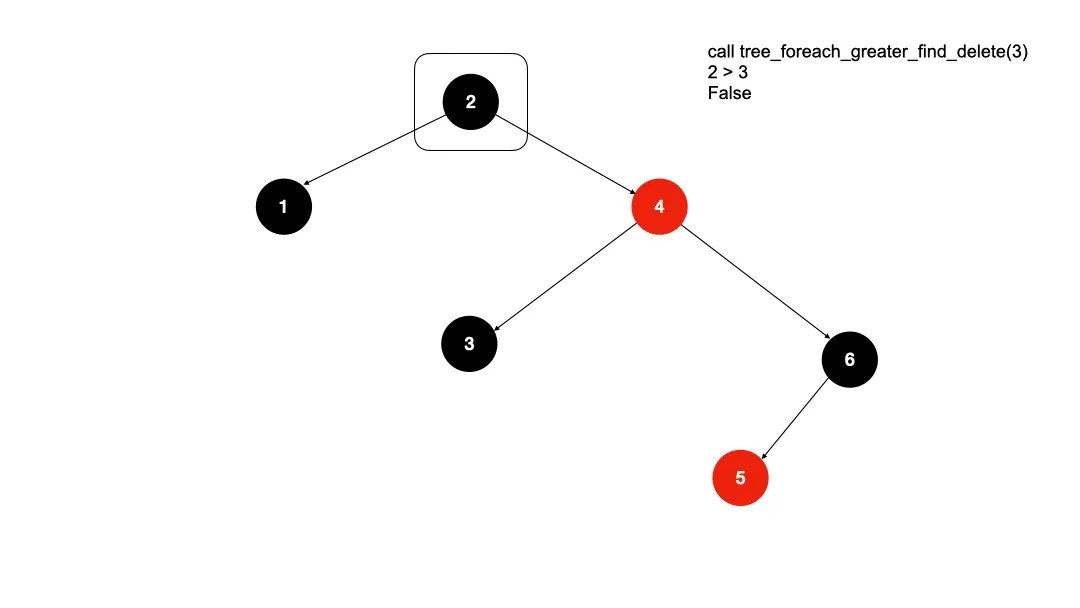
\ The keys 5 and 4 have been swapped.
\ When the cursor is on the node 4, it knows about only 3 and 6 branches. Then, during this period, the tree’s scan can't find a node. The loop can be rechecking the tree until it has at least one irrelevant key. This process isn’t slow as the keys can be found within logarithm time.
\ The expiration is time-dependent, so the application can use timestamp as a key and initiate scanning the tree when it is necessary. This method is a highly efficient way to find any expired elements.
\ For example, the code above produces the following results:
            index='16', city='Cairo', color=RED
          index='15', city='Ankara', color=BLACK
        index='14', city='Warsaw', color=RED
          index='13', city='Kyoto', color=BLACK
      index='12', city='Yokohama', color=BLACK
          index='11', city='Zhengzhou', color=BLACK
        index='10', city='Hamburg', color=RED
          index='9', city='Berlin', color=BLACK
    index='8', city='Tashkent', color=RED
        index='7', city='Waterloo', color=BLACK
      index='6', city='London', color=BLACK
        index='5', city='Istanbul', color=BLACK
  index='4', city='Beijing', color=BLACK
      index='3', city='Sydney', color=BLACK
    index='2', city='Osaka', color=BLACK
      index='1', city='New York', color=BLACK
> check elem 4
>> to delete index='4', city='Beijing'
>> to delete index='2', city='Osaka'
>> to delete index='1', city='New York'
>> to delete index='3', city='Sydney'
> check elem 8
>> to delete index='8', city='Tashkent'
>> to delete index='6', city='London'
>> to delete index='7', city='Waterloo'
> check elem 12
> check elem 9
>> to delete index='9', city='Berlin'
> check elem 10
>> to delete index='10', city='Hamburg'
> check elem 11
>> to delete index='11', city='Zhengzhou'
> check elem 5
>> to delete index='5', city='Istanbul'
> check elem 12
> check elem 12
        index='16', city='Cairo', color=RED
      index='15', city='Ankara', color=BLACK
    index='14', city='Warsaw', color=RED
      index='13', city='Kyoto', color=BLACK
  index='12', city='Yokohama', color=BLACK
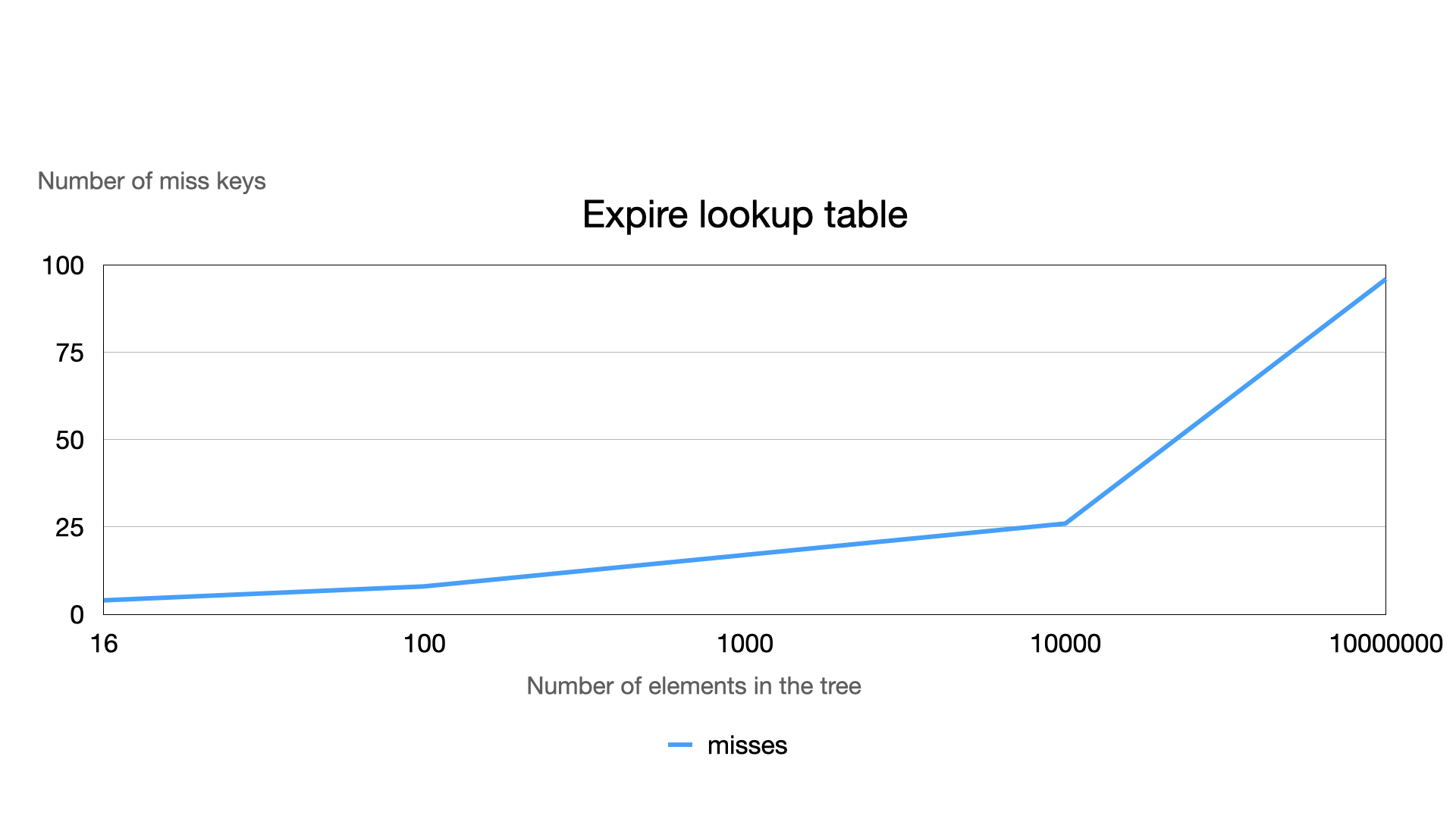
\ There are only 4 misses while looking for 11 elements in the data structure with 16 nodes. The result isn’t so optimal (3 scans with 1 miss on each). However, increasing the number of nodes in the tree makes more efficient results:
- 8 misses in 100-node tree to delete 11 expired keys (3 scans)
- 17 misses in 1000-node tree to delete 11 expired keys (3 scans)
- 26 misses in 10000-node tree to delete 11 expired keys (3 scans)
- 16 misses in 10000-node tree to delete 1000 expired keys (3 scans)
- 96 misses in 10000000-node tree to delete 1000 expired keys (6 scans)
\ This number means M * log(2)N, where N is the number of elements in the tree, and M is the total number of scan runnings. Theoretically, this number can be larger, but practically, it’s not so significant.
\
Prefix-matching trees
However, trees are used not only for requests of exact, less or greater keys. Certain types of trees have the capability to match specific parts of keys.
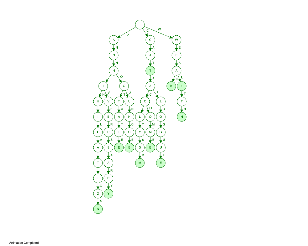
\ For instance, consider the Trie - prefix tree, a well-known data structure for finding samples by prefix or suffix. In the Trie, each node stores the letter of the word and has a number of branches equal to the count of letters in the alphabet. Therefore, the Trie can be visualized as:
 \n
\n
All nodes that are at the end of the word are marked as terminating nodes. The trie allows us to retrieve all words with a particular prefix or suffix. While searching for a prefix in the Trie, the application moves the Trie letter by letter and then scans all subsequent trie nodes from that point. As a result, searching for the prefix “wea” gives at least two resulting words: “weak” and “wealth”. Results depend on the dictionary which was loaded in the trie.
\ I’m providing another example below which involves improving the speed of search for many substrings in a string with trie. It needs to load all substring into the trie. By checking one letter at a time, the application can find multiple prefixes of the word simultaneously.
\ I suggest considering the task of searching for IP addresses inside a list of networks. This is a task of proxy-servers to identify the location of an ongoing request or analyze all traffic and its associations.
\ What if to try to use IP octets as a key? It’s an efficient decision, but it doesn’t work with subnets. Consider the network CIDRs:
- 127.0.0.0/8 - this works well as the Trie only needs to match the first octet 127.
- 192.168.0.0/16 - this also works
- 172.16.0.0/12 - this doesn’t work because this network extends from 172.16.0.0 to 172.31.255.255
\ As a result, only /8, /16 and /24 work well with a Trie. In other cases we must calculate the real position of the host in the subnet. For instance, 192.168.0.128/28 and others must use prefix matching with the calculation like an RB tree. We can combine two approaches to navigate through the tree.
\ In the picture below there is an implementation of Radix trie which is called Patricia tree. Radix trie is an optimized implementation of the trie representing a binary tree of searching that is sorted in height by the sequence of bites and sorted in width by value.
\ Patricia tree can work with bits to analyze IP Lookup Tables. It's a compressed and balanced tree. In the center all elements are centered and start from network 128.0.0.0/1 which is a central address in IPv4.
\

\n
The height of the tree depends on the smallest subnet stored in the tree. For example, if the network has only not more than /3 networks, then the tree will have only 4 levels. Otherwise, if it has the subnet with /24 mask prefix in the tree, it will have 25 levels.
\ One of the great advantages of the Patricia tree for subnet lookup - it doesn’t require storing a key. It’s easy to calculate with subnet masks by a binary operation. The binary operator AND is a common comparator in this binary tree, which is very fast.
\ Let's show an example of code representing a node and the tree:
typedef struct rnode {

    struct rnode *left;
    struct rnode *right;
    void *data;
} rnode;
typedef struct patricia_t {
    rnode *root;
} patricia_t;
\ The node doesn’t store a key and only occupies 24 bytes in memory. For 10 millions subnets it uses only 228MB.
\ Even though a hash table is a good decision for matching networks, when it comes to big sizes it increases the memory consumption. If the application stores only one byte in any node, it would require 4GB memory to store all addresses. Therefore, Trie is a good decision to store subnets because it can store only prefixes, which doesn’t increase the memory consumption so much.
A brief explanation of the comparison function
It involves a bitwise operator AND, which compares each bit of the number and generates a new number. When both bits of two numbers are equal 1, then the new number will also be 1, otherwise 0. Let's look at this with a previous example of checking IP in the network 172.16.0.0/12.
\ Let’s consider an IP 172.31.123.80.
\ In binary form, it is 10101100.00011111.01111011.01010000
\ The subnet address is 172.16.0.0/12. In the binary format this is: 10101100.00010000.00000000.00000000
\ Mask /12 means that the first 12 bits of the mask are set to 1 and the others are set to 0. This is an alternative representation of the subnet mask 255.240.0.0. In binary it is represented as:
\ 11111111.11110000.00000000.00000000
\ Check the result:
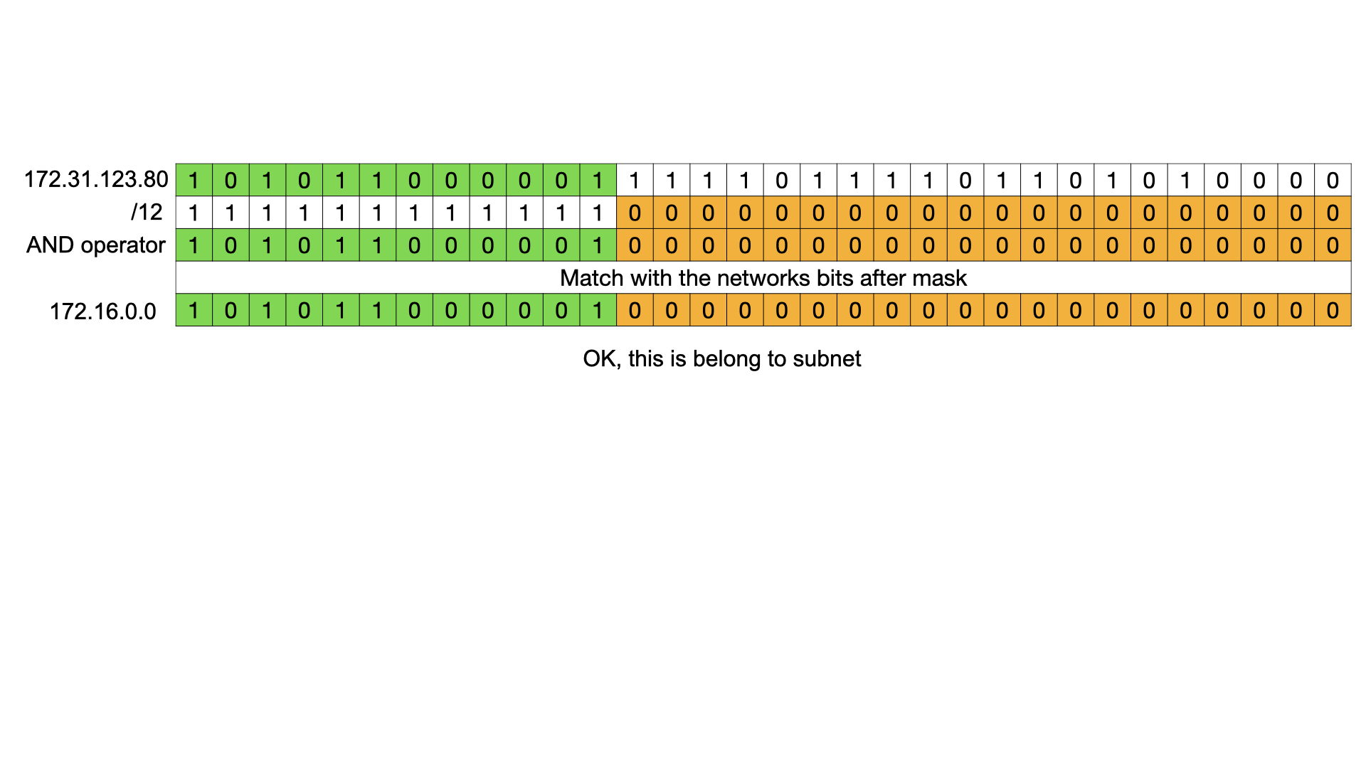
\n During each operation we can check if the IP belongs to the network from large networks to small. A found smallest network will be identified as a resulting subnet for the IP address.
\ Here is the function to insert new subnets:
rnode *patricia_insert(patricia_t *tree, uint32_t key, uint32_t mask, void *data) {
    if (!tree->root)
        tree->root = patricia_node_create();

    rnode *node = tree->root;
    rnode *next = node;

    uint32_t cursor = 0x80000000;

    while (cursor & mask) {
        if (key & cursor)
            next = node->right;
        else
            next = node->left;

        if (!next)
            break;

        cursor >>= 1;
        node = next;

    }

    if (next) {
        if (node->data) {
            return NULL;
        }

        node->data = data;
        return node;
    }

    while (cursor & mask) {
        next = patricia_node_create();

        if (key & cursor)
            node->right = next;
        else
            node->left = next;

        cursor >>= 1;
        node = next;
    }
    node->data = data;
    return node;
}
\ To lookup:
void *patricia_find(patricia_t *tree, uint32_t key)
{
    rnode *node = tree->root;
    rnode *next = node;
    rnode *ret = NULL;

    uint32_t cursor = 0x80000000;

    while (next) {
        if (node->data) {
            ret = node;
        }

        if (key & cursor) {
            next = node->right;

        } else {
            next = node->left;
        }

        node = next;
        cursor >>= 1;
    }
    return ret;
}
\ Let’s test it! I’ve found the GitHub repository “country-ip-blocks” with over 150000 subnets for detecting the country and loaded this:
\
uint32_t grpow(uint32_t basis, uint64_t exponent)
{
        uint32_t ret = basis;
        if (!exponent)
                return 1;
        else if (exponent == 1)
                return basis;

        while (--exponent)
                ret *= basis;

        return ret;
}


uint32_t ip_to_integer(char *ip, char **ptr) {
        char *cur = ip;
        uint32_t ret = 0;
        uint16_t exp = 10;
        int8_t blocks = 4;
        uint32_t blocksize = 256;

        while (--blocks >= 0)
        {
                uint16_t ochextet = strtoull(cur, &cur, exp);
                uint8_t sep = strcspn(cur, ".:");
                if (cur[sep] != '.')
                        blocks = 0;

                ret += (grpow(blocksize, blocks)*ochextet);

                ++cur;
        }

        if (ptr)
                *ptr = --cur;

        return ret;
}
uint32_t ip_get_mask(uint8_t prefix)
{
        return UINT_MAX - grpow(2, 32 - prefix) + 1;
}


void cidr_to_ip_and_mask(char *cidr, uint32_t *ip, uint32_t *mask)
{
        uint32_t ip_range;
        uint32_t ip_network;
        char *pref;
        *ip = ip_to_integer(cidr, &pref);
        uint8_t prefix;
        if (*pref == '/')
                prefix = strtoull(++pref, NULL, 10);
        else
                prefix = 32;

        if (mask)
            *mask = ip_get_mask(prefix);
}


rnode* add_ip(patricia_t *tree, char *s_ip, char *tag) {
    uint32_t mask;
    uint32_t ip;
    cidr_to_ip_and_mask(s_ip, &ip, &mask);
    return patricia_insert(tree, ip, mask, tag);
}

uint32_t fill_networks (patricia_t *tree, char *dir) {
    struct dirent *ipdirent;
    DIR *ipdir = opendir(dir);

    uint32_t count = 0;
    char fname[255];
    size_t dirlen = strlen(dir);
    strcpy(fname, dir);
    while ((ipdirent = readdir(ipdir))) {
        char *countryname = strndup(ipdirent->d_name, strcspn(ipdirent->d_name, "."));

        strcpy(fname+dirlen, ipdirent->d_name);
        FILE *fd = fopen(fname, "r");

        char buf[64];
        while (fgets(buf, 63, fd)) {
            buf[strlen(buf) - 1] = '\0';
            if(add_ip(tree, buf, countryname))
                ++count;
        }
    }

    return count;
}
\ Then, use it in the main function:
    uint32_t added = fill_networks(tree, "country-ip-blocks/ipv4/");
    printf("%u networks were added\n", added);
\ It spent only 0.01s.
\ Then, we must check the find function. It is necessary to start from small tests to make sure the tree works well:
void check_ip(patricia_t *tree, char *ip) {
    uint32_t int_ip;

    cidr_to_ip_and_mask(ip, &int_ip, NULL);
    rnode *node = patricia_find(tree, int_ip);
    if (node && node->data)
        printf("network for %s: %s\n", ip, (char*)node->data);
    else
        printf("can't find %s\n", ip);
}
\ here is the main function:
    add_ip(tree, "1.97.34.0/24", "testnet");
    add_ip(tree, "127.0.0.0/8", "localnet");
    add_ip(tree, "192.168.0.0/16", "homenet");
    add_ip(tree, "172.16.0.0/12", "compnet");
    add_ip(tree, "10.0.0.0/8", "corpnet");
    check_ip(tree, "1.97.32.34");
    check_ip(tree, "139.15.177.136");
    check_ip(tree, "209.85.233.102");
    check_ip(tree, "127.1.23.23");
    check_ip(tree, "172.17.198.23");
\ Then run:
network for 1.97.32.34: kr
network for 139.15.177.136: de
network for 209.85.233.102: us
network for 127.1.23.23: localnet
network for 172.17.198.23: compnet
It works well.
\ Check the speed:
    uint64_t count = 0;
    for (uint32_t a = 0; a < 16777216; ++a) {
        uint32_t int_ip = a;
        rnode *node = patricia_find(tree, int_ip, &count);
    }
    printf("elapsed: %lu\n", count);
\ It also took only 0.01 seconds. That’s fast enough. The Patricia tree makes it possible to find more than 16 millions IP much less than 1s. I’ve attempted to add a counter which counts the number of elements, which the application traverses through the tree. On each turn of the cycle the counter increases. In total, finding 16777216 IP addresses takes only 134217728 steps. That’s an average of 8 steps per key. It explains such a fast speed.
\
Overall about the trees
Trees are a class of data structures that can be ordered in different ways to enhance possibilities in various applications.
\ In the article we examined the Binary Trees, but this is not all of them. For instance, the AVL tree is working similarly to RB but has additional operations on insertion or deleting while maintaining better balance. On the other hand, B and B+ trees, unlike RB trees, store more than two elements in each node, which improves data locality and reduces the tree height. This improves data locality and can be useful for processor cache working or to store data on the disk. It makes B and B+ useful trees more useful as disk-stored data structures than RB or AVL. Let’s show it on the data locality:

\ There are 46 elements stored in the only 3 lines of the B-tree. RB trees make 6 lines to store the same amount of the elements. Searches find elements in 3 steps.
\ Increasing locality of data can also improve performance. For instance, processor’s cache controller retrieves the data from memory proactively more than it is necessary. Arrays stored in the memory are sequential - from 0 to N byte. Binary trees are different - every element distributed on whole memory without any guarantees. Organization of data in memory significantly impacts this process. As a result, the processor’s cache controller can get more data from the memory with an array for 1 request than in the binary trees. Modern x86 processors have L1 cache lines sized as 64 bytes. There is a reason to store elements with size 64 bytes. \n
But if the size of each element is greater than the cache line this can decrease the speed. It’s important to notice.
\ The next example connected to the disk-stored structures. Disks store information in sectors and sectors as atomic size of data which can be written or read from the disk. Old disks have a sector with 512 bytes, the modern ones - 4KB. Therefore, writing or reading 512 and 4KB takes the same amount of time.
\ Amount of reading is also an important characteristic. The more data can be read for every I/O operation from the disk, the more performance the application will have. In this case tall binary trees are not the most reasonable.
\ Therefore, RB and AVL trees are useful for the memory-stored data structure, B and B+ tree are more useful for disk-stored data structures
\ Furthermore, specialized trees like KD-tree and R-tree are designed for a specific type of data organization, such as geospatial data. This can find the points on the multidimensional space, or it can also find the near objects to the point.
Conclusions
Modern applications have the flexibility to organize the data in the memory or on disk using various methods.
\ Trees are not as fast as a hash table, but it is quite fast. Most trees ensure the logarithmic time to access the number of elements.
\ One of the key advantages of trees is their natural order. This ensures speed and precision in operations for matching elements through inexact queries.
\
There can be operations like “more than”, or “less than” in RB or B trees: \n 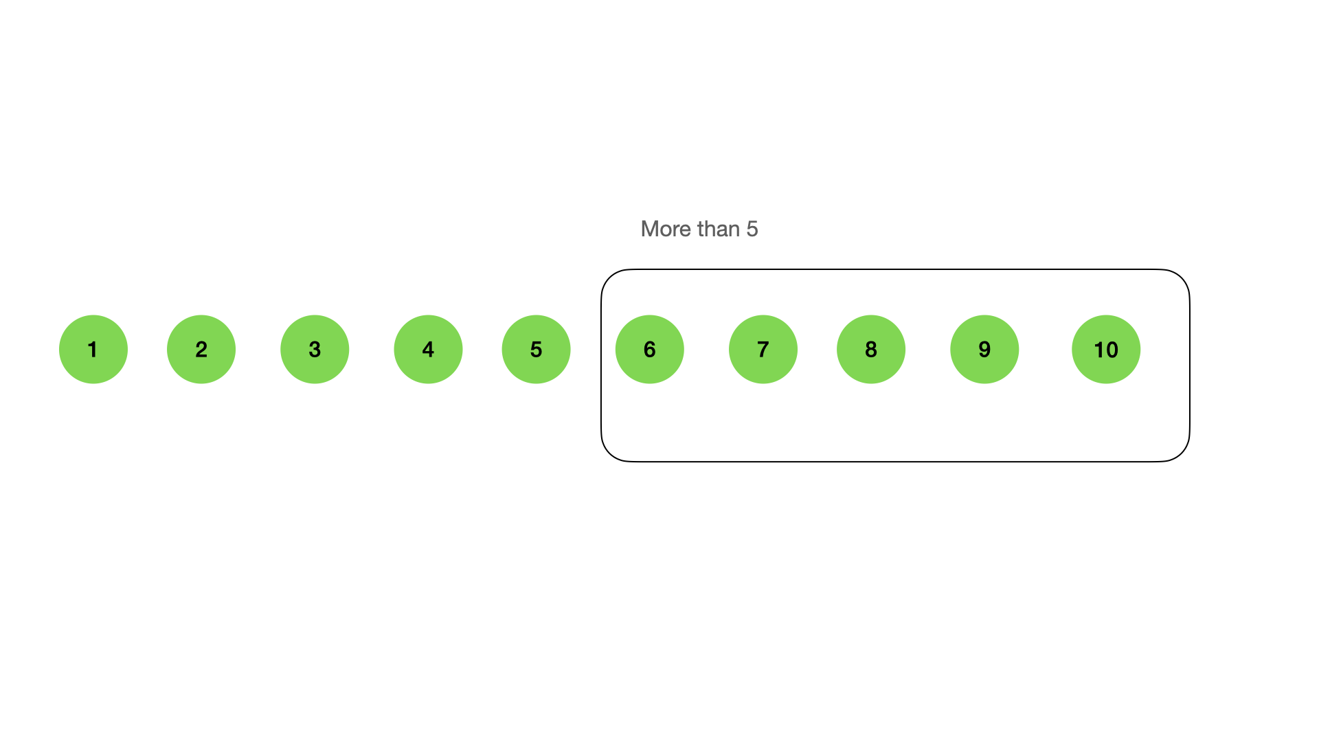 \n \n
\n \n

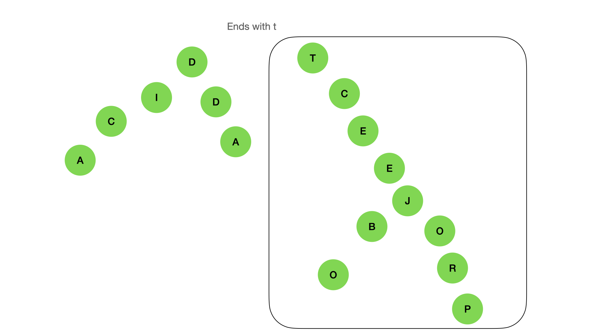
\ It also can find the nodes by prefix or suffix:
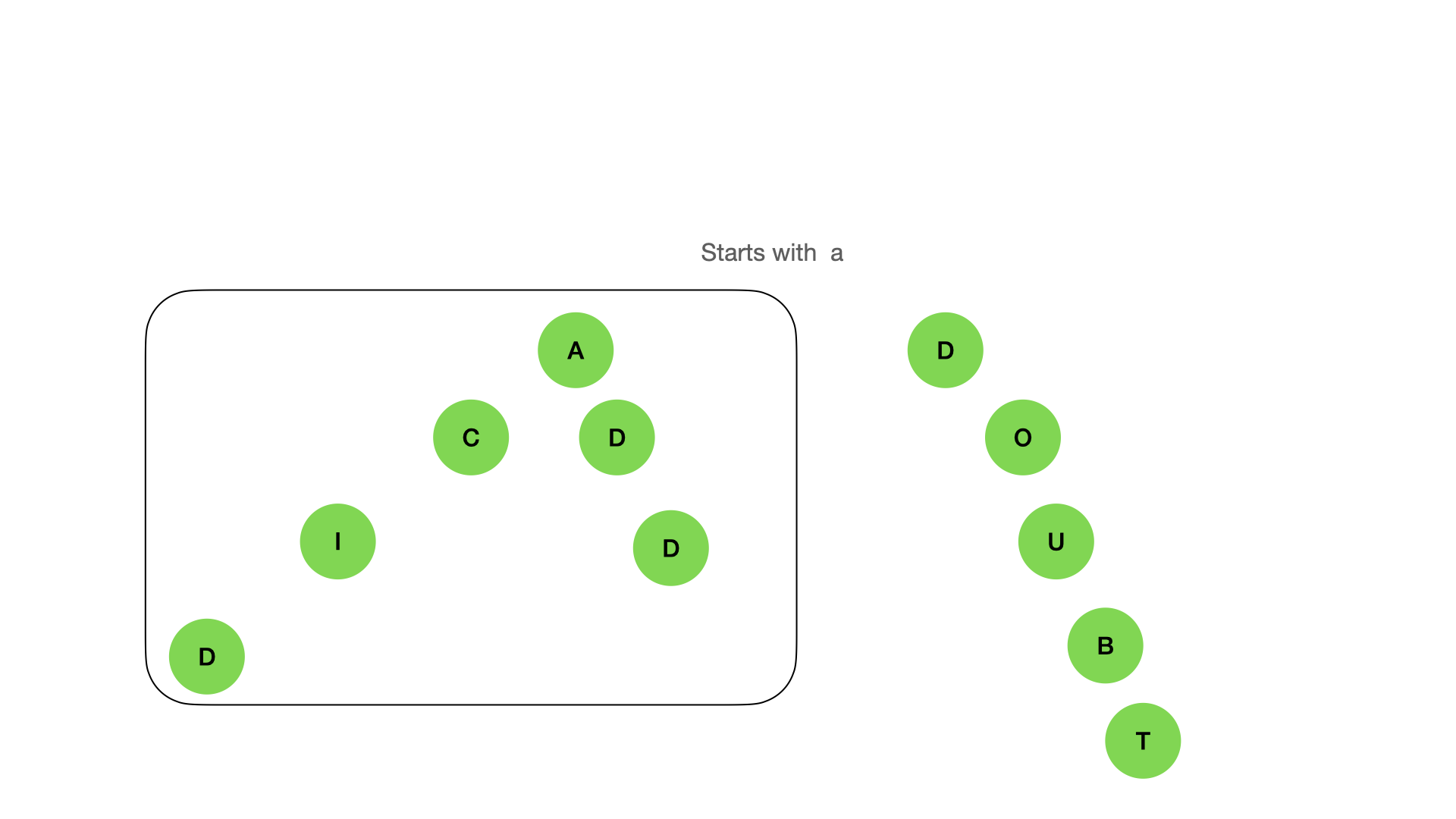
\
\ \ Or even it can find near elements:
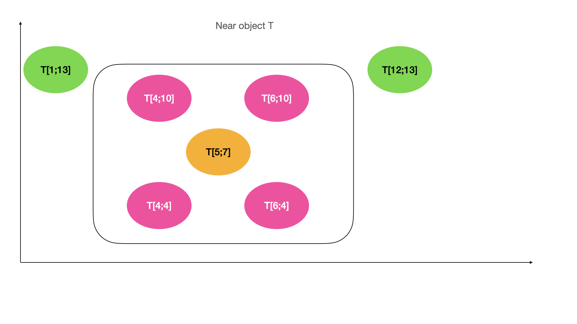
\ \ Augmenting of tree structure allows us to adapt to various scenarios. We can change the key and comparator and make it possible to store sorted elements with one or multikey. Changing mechanics of insert we can modify the tree from strings-store to subnets store. Some augmentations can improve applications performance, other - compress the data stored in the memory.
\ In general, I think that common trees only serve as a starting point to make our own data structures most suitable for specific cases. For systems that require speed, real-time processing or which operate with big arrays, data augmenting trees are a way to enhance performance of an application.
\ Choosing the standard tree and creating custom ones can distinguish one application from others. Base data structures merely provide a frame for creating something new and free from unnecessary operations and capable of performing tasks via the most efficient route.
This content originally appeared on HackerNoon and was authored by Kashintsev Georgii
Kashintsev Georgii | Sciencx (2024-07-26T15:04:38+00:00) Augmented Tree Data Structures. Retrieved from https://www.scien.cx/2024/07/26/augmented-tree-data-structures/
Please log in to upload a file.
There are no updates yet.
Click the Upload button above to add an update.
