This content originally appeared on Level Up Coding - Medium and was authored by Lu Zhenna
Summary
This article provides a beginner friendly hands-on guide to semi-supervised active learning on image classification. Active learning can train a machine learning model using fewer annotated data which drastically reduce the cost of training.
Target Audience
- Data scientists, machine learning engineers or algorithm engineers who need hands on experiences with semi-supervised machine learning.
- AI researchers who lack industrial work experiences but plan to transition into the industry.
Outline
- What is semi-supervised learning?
- What is active learning?
- Hands-on coding
For experienced data scientists, you may refer to the original tutorial on scikit learn official website. If it is too much for you to understand, this article will break it down and explain every step.
- What is semi-supervised learning?
Machine learning is broadly divided into supervised learning and unsupervised learning that most people should be familiar with. The former is machine learning with labeled training set, whereas the latter does not have any annotated data for training. Intuitively, semi-supervised learning sits somewhere in between.
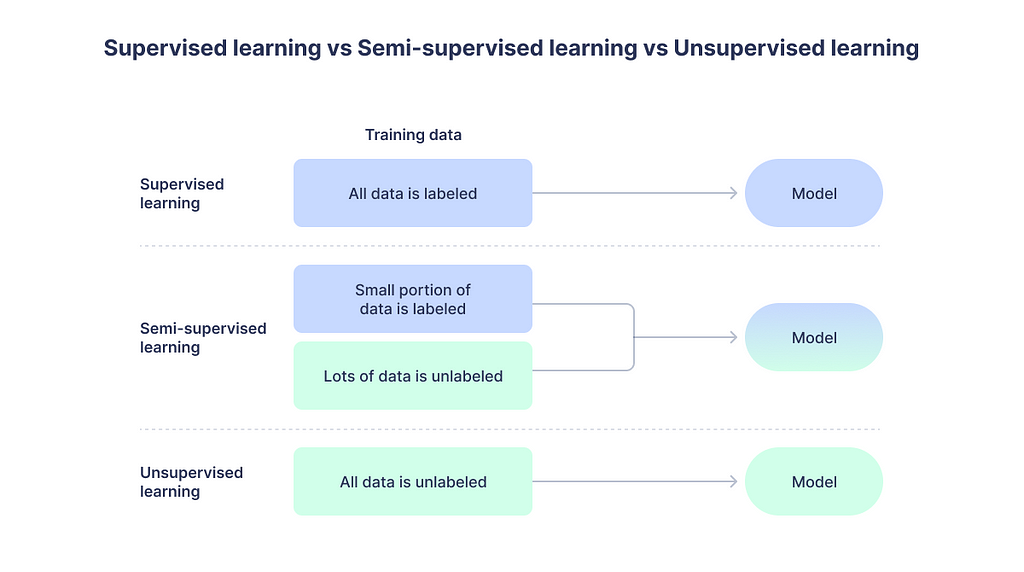
There is a huge gap between academic research and industrial applications of the algorithms. Researchers usually developed algorithms using well-annotated data. Thankfully, we have many open-source datasets for training. However, engineers in the real world have to hire people to label data before they can train a model. Data is cheap most of the time, but annotation can be quite expensive. Many data professionals will face the problem of having some labeled data but it is way too messy or insufficient to fit a good model. That’s why semi-supervised learning will have a huge market.
2. What is active learning?
Simply put, active learning is a technique that trains a machine learning model using fewer but the most informative data samples. Multiple iterations of training are required. The most informative unlabeled data samples will be selected for annotation, by a human annotator or an algorithm, after every training iteration. It efficiently reduces the amount of annotation data to train a model, which means it will SAVE A LOT OF MONEYYY!

Semi-supervised learning has a variety of algorithms that can achieve the goal of training a model with comparative level of performance using fewer labels. This field is still expanding with never-ending breakthroughs in research.
3. Hands-on coding
Please load all libraries before we start coding.
# Authors: The scikit-learn developers
# SPDX-License-Identifier: BSD-3-Clause

import matplotlib.pyplot as plt
import numpy as np
from scipy import stats

from sklearn import datasets
from sklearn.metrics import classification_report, confusion_matrix
from sklearn.semi_supervised import LabelSpreading
Then, let’s load the MNIST dataset, also known as the optical recognition of handwritten digits dataset.
digits = datasets.load_digits()
This is a scikit learn dataset that does not require any preprocessing and hence can be used directly. The feature set of digits :digits.data is a (1797, 64) array with 64 pixel features and 1797 images or data samples. (Please note that the original MNIST dataset has a train set size of 60K and a test size of 10K.) The label set of digits: digits.target is a (1797,) array with 1797 labels.
To make this experiment faster, let’s take only 330 images and shuffle them.
# shuffle data sequence
rng = np.random.RandomState(0)
indices = np.arange(len(digits.data))
rng.shuffle(indices)

# get 330 subset
X = digits.data[indices[:330]]
y = digits.target[indices[:330]]
images = digits.images[indices[:330]]
Next part may sound confusing, so please read carefully. The first iteration will start with model training using 40 out of 330 labeled data samples. In other words, let’s pretend that we ONLY have 40 labeled sample images of hand-written digits.
n_total_samples = len(y)
n_labeled_points = 40
max_iterations = 5

unlabeled_indices = np.arange(n_total_samples)[n_labeled_points:]
For the first iteration, we have 40 labeled and 290 unlabeled images. This is implemented by changing the label for these 290 images to -1.
y_train = np.copy(y)
y_train[unlabeled_indices] = -1
Let’s fit a model!
lp_model = LabelSpreading(gamma=0.25, max_iter=20)
lp_model.fit(X, y_train)
Since no changes were made to the original label set y, we can use it as ground truth to evaluate the performance of the first model.
predicted_labels = lp_model.transduction_[unlabeled_indices]
true_labels = y[unlabeled_indices]
Using classification_report, the overall accuracy is 0.87 for iteration 1.
classification_report(true_labels, predicted_labels)

Below is the confusion matrix for a clearer contrast of true positives and the rest.
cm = confusion_matrix(true_labels, predicted_labels, labels=lp_model.classes_)

Next iteration will be tough. We only have time and budget to annotate 5 images, how should we choose? Probably we should go with the least confident predictions. For now, entropy will be used as the uncertainty measure. Every image will produce a prediction distribution instead of a discrete prediction. Higher entropy means higher uncertain. It can help the model to grasp the most distinct features of the data.
# compute the entropies of transduced label distributions
pred_entropies = stats.distributions.entropy(lp_model.label_distributions_.T)

# select up to 5 digit examples that the classifier is most uncertain about
uncertainty_index = np.argsort(pred_entropies)[::-1]
uncertainty_index = uncertainty_index[
    np.isin(uncertainty_index, unlabeled_indices)
][:5]
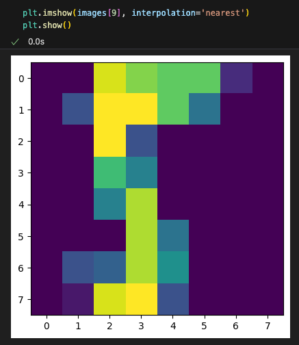
To give you a sense of what uncertainty is about, shall we get the idx of the most uncertain and least uncertain image?
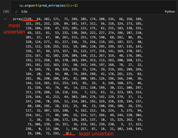
Below is the most uncertain image. Can you tell it is 1? It looks like a { to me.
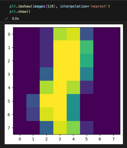
Let’s try the least uncertain image. This is a 5. Actually most of the confident predictions are 5s. Is 5 the most distinct digit? I don’t know.
Here is the most important part. We will pick the top 5 uncertain images based on entropy measures and “recover” the labels to simulate the scenario that a human annotator has labeled these 5 images. This step can be simply implemented by removing the uncertainty_index from the unlabeled_indices. Make sense? Or no?
# keep track of indices that we get labels for
delete_indices = np.array([], dtype=int)

for index, image_index in enumerate(uncertainty_index):
    image = images[image_index]

    # labeling 5 points, remote from labeled set
    (delete_index,) = np.where(unlabeled_indices == image_index)
    delete_indices = np.concatenate((delete_indices, delete_index))

unlabeled_indices = np.delete(unlabeled_indices, delete_indices)
n_labeled_points += len(uncertainty_index)
Instead of 290 unlabeled images from the start, we have 285 unlabeled images after the first iteration after “labeling 5 uncertain data samples”. We will repeat for 5 iterations.

Let’s combine all the steps and start iteration 2.
y_train = np.copy(y)
y_train[unlabeled_indices] = -1

lp_model = LabelSpreading(gamma=0.25, max_iter=20)
lp_model.fit(X, y_train)

predicted_labels = lp_model.transduction_[unlabeled_indices]
true_labels = y[unlabeled_indices]

cm = confusion_matrix(true_labels, predicted_labels, labels=lp_model.classes_)
print("Confusion matrix")
print(cm)

# compute the entropies of transduced label distributions
pred_entropies = stats.distributions.entropy(lp_model.label_distributions_.T)

# select up to 5 digit examples that the classifier is most uncertain about
uncertainty_index = np.argsort(pred_entropies)[::-1]
uncertainty_index = uncertainty_index[
    np.isin(uncertainty_index, unlabeled_indices)
][:5]

# keep track of indices that we get labels for
delete_indices = np.array([], dtype=int)

for index, image_index in enumerate(uncertainty_index):
    image = images[image_index]

    # labeling 5 points, remote from labeled set
    (delete_index,) = np.where(unlabeled_indices == image_index)
    delete_indices = np.concatenate((delete_indices, delete_index))

unlabeled_indices = np.delete(unlabeled_indices, delete_indices)
n_labeled_points += len(uncertainty_index)
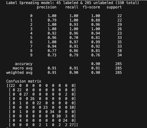
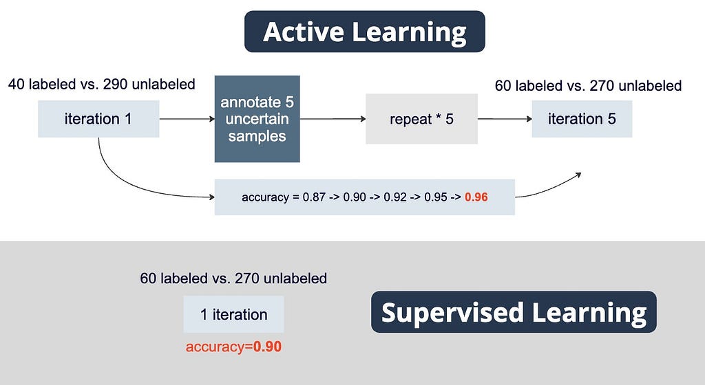
This is the performance of iteration-2 model. The accuracy increased from 0.87 to 0.90.
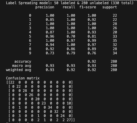
Iteration 3: the accuracy increased from 0.90 to 0.92.
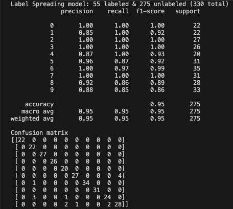
Iteration 4: the accuracy increased from 0.92 to 0.95.
Iteration 5: the accuracy increased from 0.95 to 0.96.

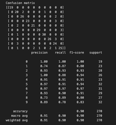
If you are not impressed, let’s directly train a model using 60 labeled images out of 330.
unlabeled_indices = np.arange(n_total_samples)[60:]

y_train = np.copy(y)
y_train[unlabeled_indices] = -1

lp_model = LabelSpreading(gamma=0.25, max_iter=20)
lp_model.fit(X, y_train)

predicted_labels = lp_model.transduction_[unlabeled_indices]
true_labels = y[unlabeled_indices]

cm = confusion_matrix(true_labels, predicted_labels, labels=lp_model.classes_)
print("Confusion matrix")
print(cm)
print(classification_report(true_labels, predicted_labels))
The performance is only 0.90 which is lower than 0.96 using active learning.
For a visual representation of the comparison between active learning and supervised learning using exactly the same 60 labeled data samples, please see the figure below.
Please download the notebook from my GitHub repo if it helps!
For more step-by-step tutorials on machine learning algorithms, please follow me!
Follow me on LinkedIn | 👏🏽 for my story | Follow me on Medium
Step-by-step Tutorial on Semi-Supervised Active Learning: For Beginners was originally published in Level Up Coding on Medium, where people are continuing the conversation by highlighting and responding to this story.
This content originally appeared on Level Up Coding - Medium and was authored by Lu Zhenna
Lu Zhenna | Sciencx (2024-07-26T16:01:24+00:00) Step-by-step Tutorial on Semi-Supervised Active Learning: For Beginners. Retrieved from https://www.scien.cx/2024/07/26/step-by-step-tutorial-on-semi-supervised-active-learning-for-beginners/
Please log in to upload a file.
There are no updates yet.
Click the Upload button above to add an update.
