This content originally appeared on HackerNoon and was authored by Quality Assurance Career Development Resources
:::info Authors:
(1) Tinghui Ouyang, National Institute of Informatics, Japan (thouyang@nii.ac.jp);
(2) Isao Echizen, National Institute of Informatics, Japan (iechizen@nii.ac.jp);
(3) Yoshiki Seo, Digital Architecture Research Center, National Institute of Advanced Industrial Science and Technology, Japan (y.seo@aist.go.jp).
:::
Table of Links
Description and Related Work of OOD Detection
Conclusions, Acknowledgement and References
II. DESCRIPTION AND RELATED WORK OF OOD DETECTION
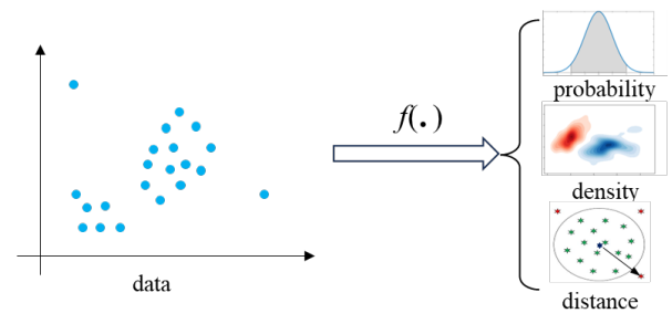
According to the idea of OOD detection methods with different statistical measures above, we can formulate the process of detecting OOD as Fig. 1.
\ Fig. 1 shows that OOD data are usually distant from the distribution of normal data and have a low density. Based on this assumption, we can easily leverage some data structural characteristics, like distribution probability, density, or
\

\ distance, to design rules distinguishing normal and outlier data. Then, the formula of OOD detection can be expressed as:
\

\ where score(·) is defined as the numeric calculation of describing a data based on a specific structural characteristic mentioned above. f(·) is the function for feature learning, e.g., kernel learning in OC-SVM and SVDD [19], deep feature learning, etc. Thus, representative features can replace the original data for better data description and OOD study. The function SM(·) is the statistical measure of the select structural characteristic, which usually calculate the difference or similarity between testing data x and the training dataset DT , e.g., KD, MD, kNN, and LOF.
\ 1) Kernel Density (KD)
\ KD estimation is developed to address the problem of nonparametric density estimation. When the natural distribution of data is hard to be described by an existing parametric probability density distribution function, the kernel function was applied for density estimation [23], as the following equation.
\

\ where, k(·, ·) is a kernel function, usually chosen as a Gaussian kernel. The kernel density (i.e., OOD score) is calculated through the average kernel distance between the testing data xt and the whole training data DT . Then, based on the idea that outliers have a lower density than normal data, we can detect OOD data based on low score values.
\ 2) Mahalanobis Distance (MD)
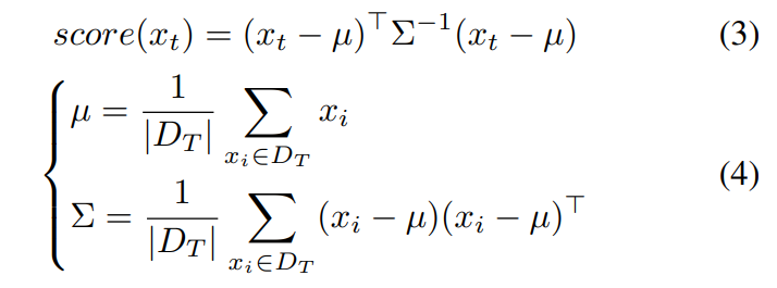
\ With the assumption of Gaussian distributed data, MD is verified as effective in defining the OOD score for anomaly detection. For example, assuming the output of the classification model in each class is approximate to be Gaussian, MD is used and verified superior in adversarial data detection [14]. The calculation of MD score is calculated below.
\

\ Based on the score of MD measurement, OOD data is assumed to have a larger distance than normal data to the center of the given data distribution.
\ 3) k-Nearest Neighbors (kNN)
\ The idea of kNN in outlier detection is similar to that of KD and MD. It mainly calculates the kNN distance and uses it for the OOD score directly, as defined below
\ where, Nk(xt) represents the k-nearest neighbors of xt. It is seen that kNN utilizes the Euclidean distance instead of the kernel distance in KD. Moreover, kNN considers the local distance as the OOD score instead of the global distance in KD and MD. Similarly, if the score of a testing data point is high, the data is assumed as OOD data.
\ 4) Local Outlier Factor (LOF) [24]
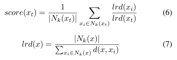
\ LOF also makes use of the local characteristic instead of the global characteristic. It describes the relative density of the testing data with respect to its neighborhood. Its calculation is first to find k-nearest neighbors of the testing data xt, then to compute the local reachability densities of xt and all its neighbors. The final score is the average density ratio of xt to its neighbors, as expressed below.
\

\ where, lrd(·) is the local reachability density function, d is the distance function. Then, under the assumption that OOD data are drawn from a different distribution than normal data, so OOD data have larger local reachability density, namely higher LOF scores.
\ Then, based on the scores calculated via different statistical measures, the rule for determining normal and outlier data can be expressed as a Boolean function, as below.
\

\ where, θ is a given threshold for OOD detection.
\
:::info This paper is available on arxiv under CC 4.0 license.
:::
\
This content originally appeared on HackerNoon and was authored by Quality Assurance Career Development Resources
Quality Assurance Career Development Resources | Sciencx (2024-08-05T23:44:16+00:00) Exploring Statistical Methods for OOD Detection: KD, MD, kNN, and LOF. Retrieved from https://www.scien.cx/2024/08/05/exploring-statistical-methods-for-ood-detection-kd-md-knn-and-lof/
Please log in to upload a file.
There are no updates yet.
Click the Upload button above to add an update.
