This content originally appeared on Level Up Coding - Medium and was authored by Harish Siva Subramanian
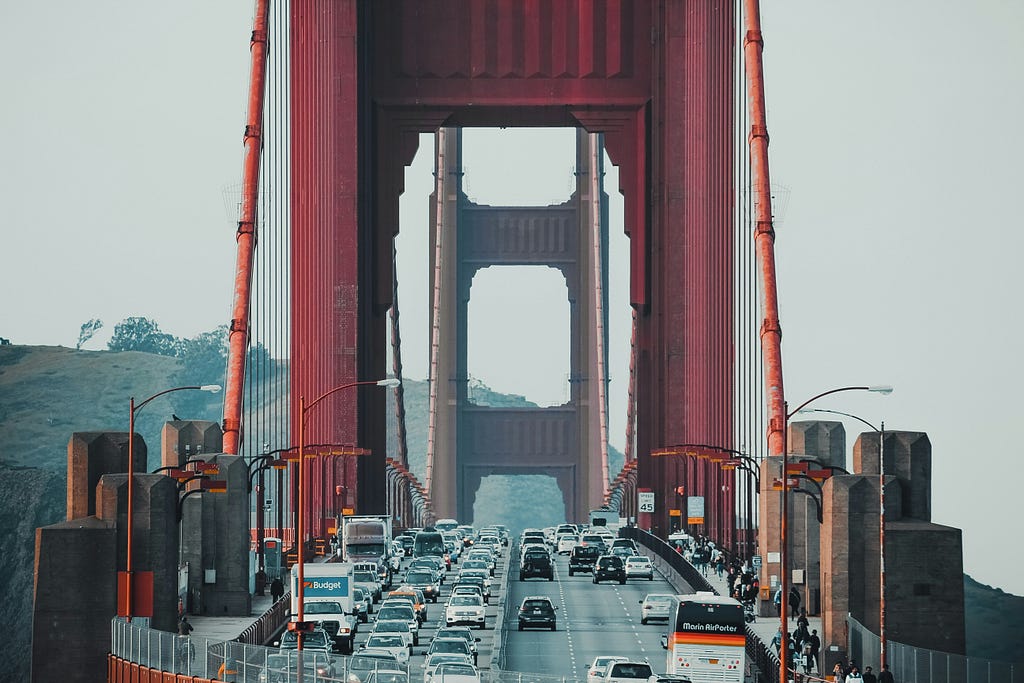
Traffic sign detection is a crucial component of Intelligent Transportation Systems (ITS) and Autonomous Vehicles (AVs), aiming to identify and classify traffic signs on roads to ensure safe and efficient traffic flow. Traffic signs, such as speed limits, traffic signals, and warning signs, convey vital information to drivers and pedestrians, and their accurate detection is essential for real-time traffic monitoring, navigation, and decision-making.
The task of traffic sign detection involves recognizing and localizing signs in images or videos captured by cameras, often under varying environmental conditions, such as lighting, weather, and camera angles. Effective traffic sign detection algorithms must be able to handle these challenges, leveraging computer vision and machine learning techniques to accurately detect and classify signs, enabling applications such as traffic monitoring, route planning, and autonomous driving.
There are many advancements in detecting the traffic signs on roads. One of the best algorithms today is the YOLO models. YOLO has achieved state-of-the-art performance on various object detection benchmarks, including the PASCAL VOC and COCO datasets, and has been widely adopted in applications such as self-driving cars, surveillance systems, and mobile devices.
First things first, lets see the implementation of YOLO V8 model to detect the traffic signs on the roads. For this purpose I obtained the dataset from the Roboflow website listed below,
Self-Driving Cars Object Detection Dataset and Pre-Trained Model by SelfDriving Car
The dataset is split to train,test and valid with each folder containing the images and their corresponding yolo formatted labels.
pip install ultralytics
This will install necessary libraries for training yolo V8.
Now its time to define the yaml file required for training.

It would contain the location of the train, test and the valid images. Also it contains the number of classes “nc” and their class names “names”.
# Import Essential Libraries
import os
import random
import pandas as pd
from PIL import Image
import cv2
from ultralytics import YOLO
from IPython.display import Video
import numpy as np
import matplotlib.pyplot as plt
import seaborn as sns
sns.set(style='darkgrid')
import pathlib
import glob
from tqdm.notebook import trange, tqdm
import warnings
warnings.filterwarnings('ignore')
Image_dir = 'train/images'

num_samples = 9
image_files = os.listdir(Image_dir)

# Randomly select num_samples images
rand_images = random.sample(image_files, num_samples)

fig, axes = plt.subplots(3, 3, figsize=(11, 11))

for i in range(num_samples):
    image = rand_images[i]
    ax = axes[i // 3, i % 3]
    ax.imshow(plt.imread(os.path.join(Image_dir, image)))
    ax.set_title(f'Image {i+1}')
    ax.axis('off')

plt.tight_layout()
plt.show()
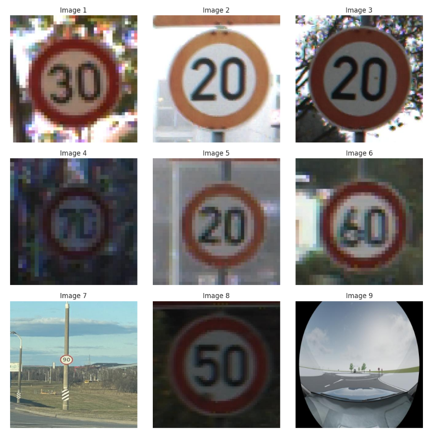
The following is a quick glimpse of the images displayed,
#Training Process
model=YOLO(model='yolov8s.pt')

if __name__=='__main__':
    model.train(data="data.yaml",epochs=15,device=0,imgsz=640)
The above script will perform the training process. Once the training is done, it is time for us to visualize the results.
import os
import cv2
import matplotlib.pyplot as plt

def display_images(post_training_files_path, image_files):

    for image_file in image_files:
        image_path = os.path.join(post_training_files_path, image_file)
        img = cv2.imread(image_path)
        img = cv2.cvtColor(img, cv2.COLOR_BGR2RGB)

        plt.figure(figsize=(10, 10), dpi=120)
        plt.imshow(img)
        plt.axis('off')
        plt.show()

# List of image files to display
image_files = [
    'confusion_matrix_normalized.png',
    'F1_curve.png',
    'P_curve.png',
    'R_curve.png',
    'PR_curve.png',
    'results.png'
]

# Path to the directory containing the images
post_training_files_path = r'C:\Users\Harish\PycharmProjects\Yolov8_TrafficSign\runs\detect\train'

# Display the images
display_images(post_training_files_path, image_files)
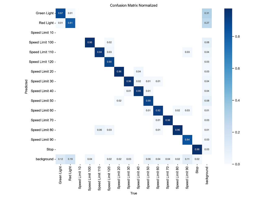
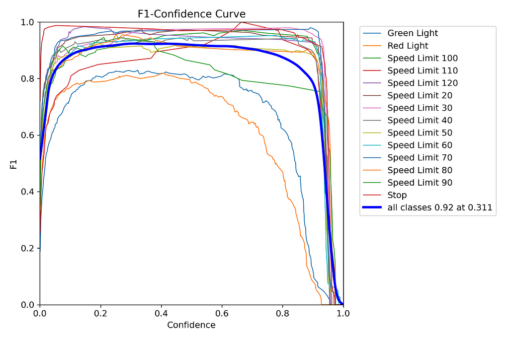
And many more figures. You can check all the figures in the folder runs/detect/train which is automatically created when you train the model.
import pandas as pd
Result_Final_model = pd.read_csv(r'C:\Users\Harish\PycharmProjects\Yolov8_TrafficSign\runs\detect\train\results.csv')
This will read the csv file from the folder created after the train run
import seaborn as sns
# Read the results.csv file as a pandas dataframe
Result_Final_model.columns = Result_Final_model.columns.str.strip()

# Create subplots
fig, axs = plt.subplots(nrows=5, ncols=2, figsize=(15, 15))

# Plot the columns using seaborn
sns.lineplot(x='epoch', y='train/box_loss', data=Result_Final_model, ax=axs[0,0])
sns.lineplot(x='epoch', y='train/cls_loss', data=Result_Final_model, ax=axs[0,1])
sns.lineplot(x='epoch', y='train/dfl_loss', data=Result_Final_model, ax=axs[1,0])
sns.lineplot(x='epoch', y='metrics/precision(B)', data=Result_Final_model, ax=axs[1,1])
sns.lineplot(x='epoch', y='metrics/recall(B)', data=Result_Final_model, ax=axs[2,0])
sns.lineplot(x='epoch', y='metrics/mAP50(B)', data=Result_Final_model, ax=axs[2,1])
sns.lineplot(x='epoch', y='metrics/mAP50-95(B)', data=Result_Final_model, ax=axs[3,0])
sns.lineplot(x='epoch', y='val/box_loss', data=Result_Final_model, ax=axs[3,1])
sns.lineplot(x='epoch', y='val/cls_loss', data=Result_Final_model, ax=axs[4,0])
sns.lineplot(x='epoch', y='val/dfl_loss', data=Result_Final_model, ax=axs[4,1])

# Set titles and axis labels for each subplot
axs[0,0].set(title='Train Box Loss')
axs[0,1].set(title='Train Class Loss')
axs[1,0].set(title='Train DFL Loss')
axs[1,1].set(title='Metrics Precision (B)')
axs[2,0].set(title='Metrics Recall (B)')
axs[2,1].set(title='Metrics mAP50 (B)')
axs[3,0].set(title='Metrics mAP50-95 (B)')
axs[3,1].set(title='Validation Box Loss')
axs[4,0].set(title='Validation Class Loss')
axs[4,1].set(title='Validation DFL Loss')


plt.suptitle('Training Metrics and Loss', fontsize=24)
plt.subplots_adjust(top=0.8)
plt.tight_layout()
plt.show()
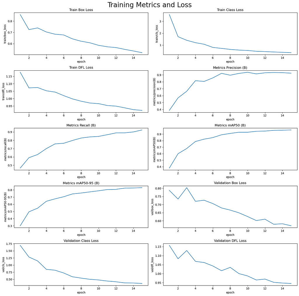
We can see the visualization of different metrics.
Now its time for us to check the validation performance metrics,
from ultralytics import YOLO
# Loading the best performing model
Valid_model = YOLO(r'C:\Users\Harish\PycharmProjects\Yolov8_TrafficSign\runs\detect\train\weights\best.pt')

if __name__=='__main__':
    # Evaluating the model on the validset
    metrics = Valid_model.val(split = 'val')

    # final results
    print("precision(B): ", metrics.results_dict["metrics/precision(B)"])
    print("metrics/recall(B): ", metrics.results_dict["metrics/recall(B)"])
    print("metrics/mAP50(B): ", metrics.results_dict["metrics/mAP50(B)"])
    print("metrics/mAP50-95(B): ", metrics.results_dict["metrics/mAP50-95(B)"])

And finally its time to make predictions on the test images.
import os
import random
import pandas as pd
from PIL import Image
import cv2
from ultralytics import YOLO
import matplotlib.pyplot as plt
import seaborn as sns
import numpy as np


# Normalization function
def normalize_image(image):
    return image / 255.0


# Image resizing function
def resize_image(image, size=(640, 640)):
    return cv2.resize(image, size)

if __name__=='__main__':
    # Path to validation images
    dataset_path = 'C:/Users/Harish/IPYNBs/YoloV8_TrafficSigns/car/'  # Place your dataset path here
    valid_images_path = os.path.join(dataset_path, 'test', 'images')

    Valid_model = YOLO(r'C:\Users\Harish\PycharmProjects\Yolov8_TrafficSign\runs\detect\train\weights\best.pt')


    # List of all jpg images in the directory
    image_files = [file for file in os.listdir(valid_images_path) if file.endswith('.jpg')]

    # Check if there are images in the directory
    if len(image_files) > 0:
        # Select 9 images at equal intervals
        num_images = len(image_files)
        step_size = max(1, num_images // 9)  # Ensure the interval is at least 1
        selected_images = [image_files[i] for i in range(0, num_images, step_size)]

        # Prepare subplots
        fig, axes = plt.subplots(3, 3, figsize=(20, 21))
        fig.suptitle('Validation Set Inferences', fontsize=24)

        for i, ax in enumerate(axes.flatten()):
            if i < len(selected_images):
                image_path = os.path.join(valid_images_path, selected_images[i])

                # Load image
                image = cv2.imread(image_path)

                # Check if the image is loaded correctly
                if image is not None:
                    # Resize image
                    resized_image = resize_image(image, size=(640, 640))
                    # Normalize image
                    normalized_image = normalize_image(resized_image)

                    # Convert the normalized image to uint8 data type
                    normalized_image_uint8 = (normalized_image * 255).astype(np.uint8)

                    # Predict with the model
                    results = Valid_model.predict(source=normalized_image_uint8, imgsz=640, conf=0.5)

                    # Plot image with labels
                    annotated_image = results[0].plot(line_width=1)
                    annotated_image_rgb = cv2.cvtColor(annotated_image, cv2.COLOR_BGR2RGB)
                    ax.imshow(annotated_image_rgb)
                else:
                    print(f"Failed to load image {image_path}")
            ax.axis('off')

        plt.tight_layout()
        plt.show()
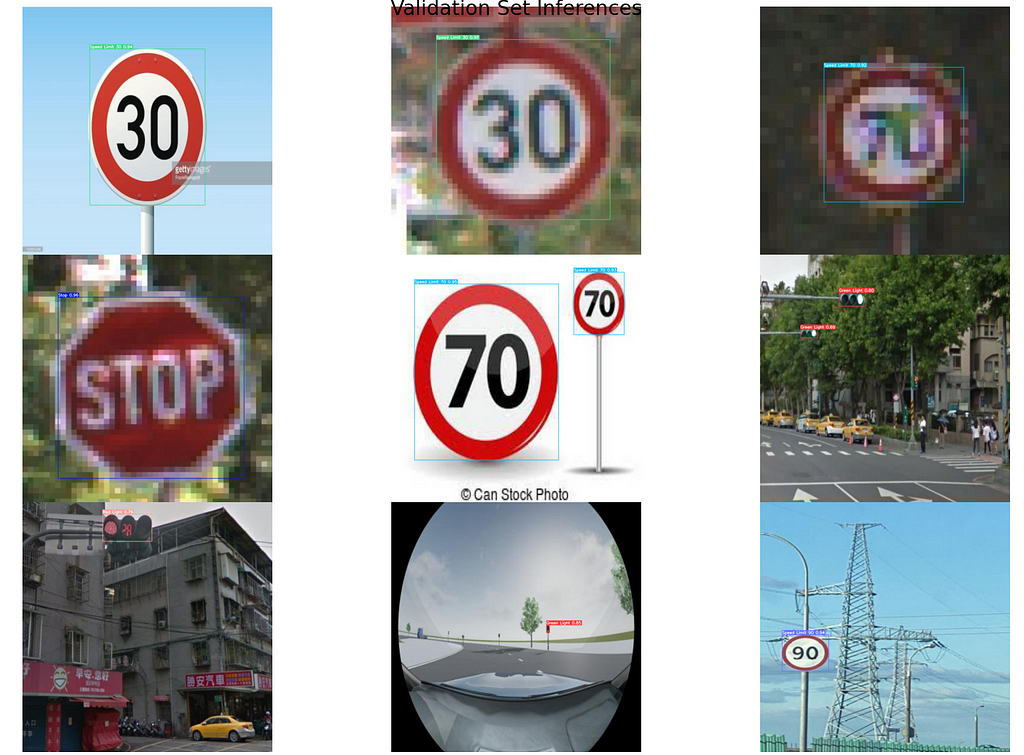
The predictions are looking great. The next step is to do the prediction for a video on each frame that can be applied to self-driving cars.
Thank you for reading!!
If you like the article and would like to support me, make sure to:
- 👏 Clap for the story (50 claps) to help this article be featured
- Follow me on Medium
- 📰 View more content on my medium profile
- 🔔 Follow Me: LinkedIn | GitHub
Traffic Signs Detection for Self Driving Cars was originally published in Level Up Coding on Medium, where people are continuing the conversation by highlighting and responding to this story.
This content originally appeared on Level Up Coding - Medium and was authored by Harish Siva Subramanian
Harish Siva Subramanian | Sciencx (2024-08-06T22:22:44+00:00) Traffic Signs Detection for Self Driving Cars. Retrieved from https://www.scien.cx/2024/08/06/traffic-signs-detection-for-self-driving-cars/
Please log in to upload a file.
There are no updates yet.
Click the Upload button above to add an update.
