
This content originally appeared on Level Up Coding - Medium and was authored by Pavlo Kolodka
Learn how to boost database efficiency and handle growth.

Introduction
As software grows, there comes a time when you need to improve the performance of data storage. This could manifest as a slowdown in search speed, a degradation in write operations, or an overall performance decrease. While understanding these challenges is critical, knowing the common approaches to address them is equally important.
In this article, I’ll try to gather all available techniques that I consider when dealing with database performance. I’ll start with simple tips and gradually introduce more complex methods as the cost of implementation increases.
This guide will be helpful for anyone who wants to expand their knowledge about databases. Grasping all of this may be challenging, but is definitely worth exploring.
Query optimization
Let’s start with the query itself. In this section, you will gain an understanding of execution order, the danger of a correlated subquery, recognizing when to apply batching and materialize view, and analyzing the execution plan.
Leverage execution order
You can tell what approximate query complexity is by looking at it. The trick here is to know the order in which SQL statements are executed.
Here is the bottom-up order of a typical SQL query execution:
- FROM
- JOIN
- WHERE
- GROUP BY
- HAVING
- SELECT
- ORDER BY
- OFFSET
- LIMIT
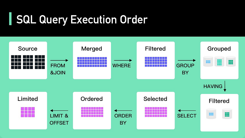
When you know the order of query execution, you understand that the earlier you apply a constraint, the more benefit you will get in terms of processing performance.
As an example, let’s consider that we have a product table with different categories, and we need to find the average price of the ‘Electronics’ category. One of the possible queries could be this:
SELECT category, AVG(price) AS avg_price
FROM products
HAVING category = 'Electronics' AND AVG(price) > 100
GROUP BY category;
But as you might have noticed, category filtration happens in the HAVING block. The downside of this is that the filtration by category will always take place after aggregation, which, with a large amount of data, may result in a significant query time increase, especially if we have an index on the category column. That’s because the HAVING clause is applied for a temporary aggregated table that, without the database optimizer, cannot use indexes for filtration (you can reveal that with the EXPLAIN command).
It’s better to apply initial filtering as early as possible to reduce processing power on aggregation and further limiting and sorting.
SELECT category, AVG(price) AS avg_price
FROM products
WHERE category = 'Electronics'
GROUP BY category
HAVING AVG(price) > 100;
Correlated subquery
As we discuss improving query performance, there is a type of subquery you need to pay attention to: a correlated subquery.
A correlated subquery is a subquery that uses values from the outer query. The drawback of such a nested query is that it will be executed for every outer row. That’s a high computation effort for a large dataset.
One of the alternatives to correlated subquery is to use JOIN. Consider the following example, where we want to find employees whose salary is above the average salary in their department:
                             Table "public.Employee"
    Column     |  Type   | Collation | Nullable |             Default
---------------+---------+-----------+----------+---------------------------------
 id            | integer |           | not null | nextval('employee_id_seq'::regclass)
 department_id | integer |           |          |
 name          | text    |           |          |
 salary        | numeric |           |          |
SELECT e1.employee_id, e1.employee_name, e1.salary
FROM employee e1
WHERE e1.salary > (
  SELECT AVG(e2.salary)
  FROM employees e2
  WHERE e2.department_id = e1.department_id
);
Let’s rewrite it using JOIN:
SELECT e1.employee_id, e1.employee_name, e1.salary
FROM employee e1
JOIN (
  SELECT department_id, AVG(salary) AS avg_salary
  FROM employee
  GROUP BY department_id
) e2 ON e1.department_id = e2.department_id
WHERE e1.salary > e2.avg_salary;
The main difference is that in the case of the correlated subquery, the average will be executed for every row from the employee table, and in the case of using JOIN, the average calculation will be executed only once. You will see the detailed difference in the query analyzing chapter.
Apply batching
One technique that can noticeably boost database execution is to apply batching when possible. When you deal with bulk operations, instead of executing individual insert, update, or delete statements, you group them together into a single batch.

This includes two major benefits:
- Reduced network latency: By sending multiple operations in a single request, you minimize the network latency that occurs with each round-trip between the client and the database server.
- Improved throughput: The database server can process the batch more efficiently than it can process many individual operations, often leading to higher throughput. That’s because, under the hood, many databases wrap operations in the transactions, which, in the case of batching, reduces the overhead of starting and committing multiple transactions.
Utilize materialized view
When you have a case of heavy computation, such as aggregates involving the combination of several tables, and that computation occurs rarely, you might consider using a materialized view.
A materialized view is very similar to a basic VIEW, except it stores its values on disk, which is the opposite of fetching data every time when you query a basic VIEW.
This is a good mechanism to implement pre-computation with a custom refresh interval. Instead of scanning thousands of rows and then processing them, you execute one SELECT query and get all the results.
Analyze query execution plan
To apply the above tips properly for a particular DBMS with a special environment, you need to understand how exactly the database will execute your query. This is because when you write a query, essentially, what you’re doing is describing what data you want to get, and the implementation details go up to the database.
One possible way to examine underlying magic is to use the EXPLAIN command. Let’s analyze the performance between previously discussed correlated and JOIN queries:
The first query using a correlated subquery:
EXPLAIN ANALYZE SELECT e1.employee_id, e1.employee_name, e1.salary
FROM employee e1
WHERE e1.salary > (
    SELECT AVG(e2.salary)
    FROM employee e2
    WHERE e2.department_id = e1.department_id
);
The output:
QUERY PLAN                                                                                                          |
--------------------------------------------------------------------------------------------------------------------+
Seq Scan on employee e1  (cost=0.00..16339.60 rows=270 width=68) (actual time=0.045..0.063 rows=4 loops=1)          |
  Filter: (salary > (SubPlan 1))                                                                                    |
  Rows Removed by Filter: 7                                                                                         |
  SubPlan 1                                                                                                         |
    ->  Aggregate  (cost=20.14..20.15 rows=1 width=32) (actual time=0.004..0.004 rows=1 loops=11)                   |
          ->  Seq Scan on employee e2  (cost=0.00..20.12 rows=4 width=32) (actual time=0.001..0.001 rows=6 loops=11)|
                Filter: (department_id = e1.department_id)                                                          |
                Rows Removed by Filter: 5                                                                           |
Planning Time: 0.153 ms                                                                                             |
Execution Time: 0.090 ms                                                                                            |                                                                                  |
The second query using the JOIN operator:
EXPLAIN ANALYZE SELECT e1.employee_id, e1.employee_name, e1.salary
FROM employee e1
JOIN (
    SELECT department_id, AVG(salary) AS avg_salary
    FROM employee
    GROUP BY department_id
) e2 ON e1.department_id = e2.department_id
WHERE e1.salary > e2.avg_salary;
The output:
QUERY PLAN                                                                                                             |
-----------------------------------------------------------------------------------------------------------------------+
Hash Join  (cost=29.15..49.39 rows=270 width=68) (actual time=0.038..0.041 rows=4 loops=1)                             |
  Hash Cond: (e1.department_id = employee.department_id)                                                               |
  Join Filter: (e1.salary > (avg(employee.salary)))                                                                    |
  Rows Removed by Join Filter: 7                                                                                       |
  ->  Seq Scan on employee e1  (cost=0.00..18.10 rows=810 width=72) (actual time=0.004..0.005 rows=11 loops=1)         |
  ->  Hash  (cost=26.65..26.65 rows=200 width=36) (actual time=0.024..0.025 rows=3 loops=1)                            |
        Buckets: 1024  Batches: 1  Memory Usage: 9kB                                                                   |
        ->  HashAggregate  (cost=22.15..24.65 rows=200 width=36) (actual time=0.015..0.017 rows=3 loops=1)             |
              Group Key: employee.department_id                                                                        |
              Batches: 1  Memory Usage: 40kB                                                                           |
              ->  Seq Scan on employee  (cost=0.00..18.10 rows=810 width=36) (actual time=0.001..0.002 rows=11 loops=1)|
Planning Time: 0.163 ms                                                                                                |
Execution Time: 0.100 ms                                                                                               |                                                                                      |
Summary of operations
1. First query (correlated subquery):
- Sequential Scan on employee e1: 1 time
- Sequential Scan on employee e2: 11 times (once for each row in employee e1)
- Aggregate Calculation: 11 times (once for each row in employee e1)
2. Second query (JOIN with aggregated subquery):
- Sequential Scan on employee e1: 1 time
- Sequential Scan on employee (for subquery): 1 time
- Hash Aggregate: 1 time
- Hash Join: 1 time
What you can see here is that in the case of the JOIN query, the average aggregation is executed once for the entire table. In contrast, the AVG function was executed 11 times for the first query — the same number of times as there are rows in the table (loops=11). Since the number of rows is very small, the time difference is minimal, but in a large dataset, the difference can be significant.
Indexes:
When facing the problem of speeding up read operations, one potential solution is to use indexing. Creating indexes is a useful choice as it does not require modifying an existing schema and can greatly improve search performance.
There are two types of indexes: clustered and non-clustered. A clustered index is mostly automatically created for a primary key, as it indicates the physical order of rows. In contrast, a non-clustered index does not necessarily reflect the actual order of data; it’s an additional list that speeds up a lookup by a certain attribute. Next, I’ll talk about non-clustered indexes.
One of the important things when working with indexes is to know when to apply them. Generally, you prioritize indexing for columns that are frequently used in query filters. In particular, they are useful with these 3 main clauses:
- WHERE
- JOIN
- ORDER BY
What’s the downside of indexes? It’s a space and write cost. Indexes reduce the number of disk I/O operations, allowing the database not to perform a full table scan by given criteria.
It’s done by creating an additional storage that holds an indexed column(s) and the pointer to the actual row. You can think about it as key-value storage, where a key is an indexed column, and the value is a reference to an actual row. In fact, the two most popular implementations of indexes include creating a B-tree (B+ tree) or a hash table. That’s the storage overhead.
The write cost means operations like INSERT, UPDATE, DELETE will take more time because, in addition to the operation itself, you need to keep the index order up-to-date.
Let’s compare a search for the employee table for a given name.
Without an index for the department column, you can see the next query plan:
EXPLAIN ANALYZE SELECT * FROM employee WHERE name = 'John';

QUERY PLAN                                                                                           |
-----------------------------------------------------------------------------------------------------+
Seq Scan on employee  (cost=0.00..18.50 rows=200 width=4) (actual time=0.010..0.097 rows=200 loops=1)|
  Filter: (name = 'John'::text)                                                                        |
  Rows Removed by Filter: 800                                                                        |
Planning Time: 0.142 ms                                                                              |
Execution Time: 0.130 ms                                                                             |
Let’s add a new index for the name attribute:
CREATE INDEX idx_employee_name
ON employee (name);
And reanalyze the query plan:
EXPLAIN ANALYZE SELECT * FROM employee WHERE name = 'John';

QUERY PLAN                                                                                                                           |
-------------------------------------------------------------------------------------------------------------------------------------+
Index Scan using idx_employee_name on employee  (cost=0.15..10.76 rows=178 width=4) (actual time=0.084..0.237 rows=178 loops=1)|
  Index Cond: (name = 'John'::text)                                                                                              |
Planning Time: 0.148 ms                                                                                                              |
Execution Time: 0.097 ms                                                                                                             |
In addition to decreased searing time, you can see the employment of the created index¹.
Note 1: In the case when multiple rows satisfy the condition, a database is likely to use a bitmap index.
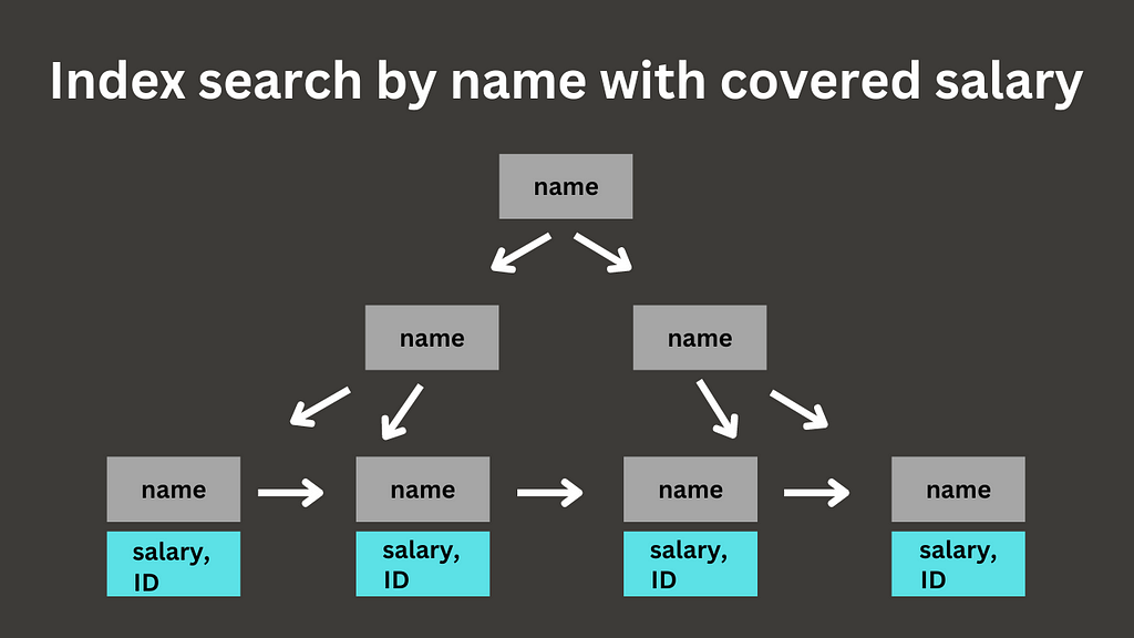
Covering indexes
What if I told you that you can speed up indexes themselves if you create them properly? The way to do it is to use covering indexes.
Suppose we want to find the salary of an employee by a given name. In the typical index search, there are two phases: index scan and table scan. When the database finds a needed index element, it’ll grab the internal ID of the row that’s stored next to the index element and perform the additional lookup on the main table using that ID.

But when you know the queried values beforehand, you can eliminate the second scan, resulting in the index-only scan. The way to do it is to create a covering index that covers all the needed columns.
Let’s conduct some tests. First of all, we will analyze a plain index search:
EXPLAIN ANALYZE SELECT salary FROM employee WHERE name = 'John';

QUERY PLAN                                                                                                                           |
-------------------------------------------------------------------------------------------------------------------------------------+
Index Scan using idx_employee_name on employee  (cost=0.15..10.72 rows=178 width=4) (actual time=0.084..0.237 rows=178 loops=1)|
  Index Cond: (name = 'John'::text)                                                                                              |
Planning Time: 0.132 ms                                                                                                              |
Execution Time: 0.095 ms
To utilize a covering index, we need to recreate an index to cover additional fields (in our case, it’s a salary attribute). There are two options for doing it: add covered attributes directly to the index or include needed columns into the index payload.
DROP INDEX idx_employee_name
CREATE INDEX idx_employee_name
ON Employee (name, salary);
And analyze the query:
EXPLAIN ANALYZE SELECT salary FROM employee WHERE name = 'John';

QUERY PLAN                                                                                                                               |
-----------------------------------------------------------------------------------------------------------------------------------------+
Index Only Scan using idx_employee_name on employee  (cost=0.28..5.59 rows=178 width=4) (actual time=0.080..0.101 rows=178 loops=1)|
  Index Cond: (name = 'John'::text)                                                                                                  |
  Heap Fetches: 0                                                                                                                        |
Planning Time: 0.136 ms                                                                                                                  |
Execution Time: 0.086 ms                                                                                                                 |
Here, we can see that Postgres successfully applied the index, resulting in the index-only scan. Also, you can observe Heap Fetches: 0, meaning Postgres did not conduct a search in the main table.

Postgres allows for the addition of covered columns into the index payload instead of indexing them directly. So, while a payload will not be used in conditional like WHERE, it will be helpful in eliminating the main table lookup.
CREATE INDEX idx_employee_name
ON Employee (name) INCLUDE (salary);

EXPLAIN ANALYZE SELECT salary FROM employee WHERE name = 'John';

QUERY PLAN                                                                                                                               |
-----------------------------------------------------------------------------------------------------------------------------------------+
Index Only Scan using idx_employee_name on employee  (cost=0.28..5.59 rows=178 width=4) (actual time=0.068..0.080 rows=178 loops=1)|
  Index Cond: (name = 'John'::text)                                                                                                  |
  Heap Fetches: 0                                                                                                                        |
Planning Time: 0.153 ms                                                                                                                  |
Execution Time: 0.075 ms                                                                                                                 |
Denormalization
There are situations when you cannot improve performance by not touching the current database scheme. It may involve adding new columns for frequently accessed or precomputed values, removing a relation table to avoid joins, or, on the contrary, creating duplicating tables to store denormalized data. Such a process is called denormalization.
Denormalization is a technique used to improve database read performance by intentionally adding data redundancy. Mainly, denormalization is utilized to remove heavy JOIN operations. By duplicating data to leverage fast access, it brings a downside in the form of increased complexity of write operations and maintaining data integrity.
To give you a concrete example, let’s imagine we have a customer table and an order table.
TABLE Order (
    id INT PRIMARY KEY,
    customer_id INT,
    date DATE
);

TABLE Customer (
    id INT PRIMARY KEY,
    name VARCHAR(100)
);
You have a simple task: to output all the orders with their related customer names. This can be done using a single JOIN by referring to the customer_id from the ‘Order’ table and matching it with the primary key of the ‘Customer’ table. It’s not too complex at this stage, but as other fields or tables are added, the computation time for fetching data from the disk and building a temporary table will increase, potentially slowing down the search query.
In the context of denormalization, the solution is to store the customer’s name directly in the ‘Order’ table so that we can query the needed information without joining tables.
TABLE Order (
    id INT PRIMARY KEY,
    customer_id INT,
    customer_name VARCHAR(100), -- Redundant column
    date DATE
);

TABLE Customer (
    id INT PRIMARY KEY,
    name VARCHAR(100)
);
Configuration adjustment
Assume you have already applied query optimization strategies, but the performance still doesn’t meet the requirements. One potential solution is to adjust the current configuration settings. Keeping the default values is not always a good idea, as your working environment may be either resource-limited or resource-wasting. Customizing settings, such as the maximum number of connections, buffer pool size, transient memory, etc., can provide the fine-tuning options you need.
Connection pooling
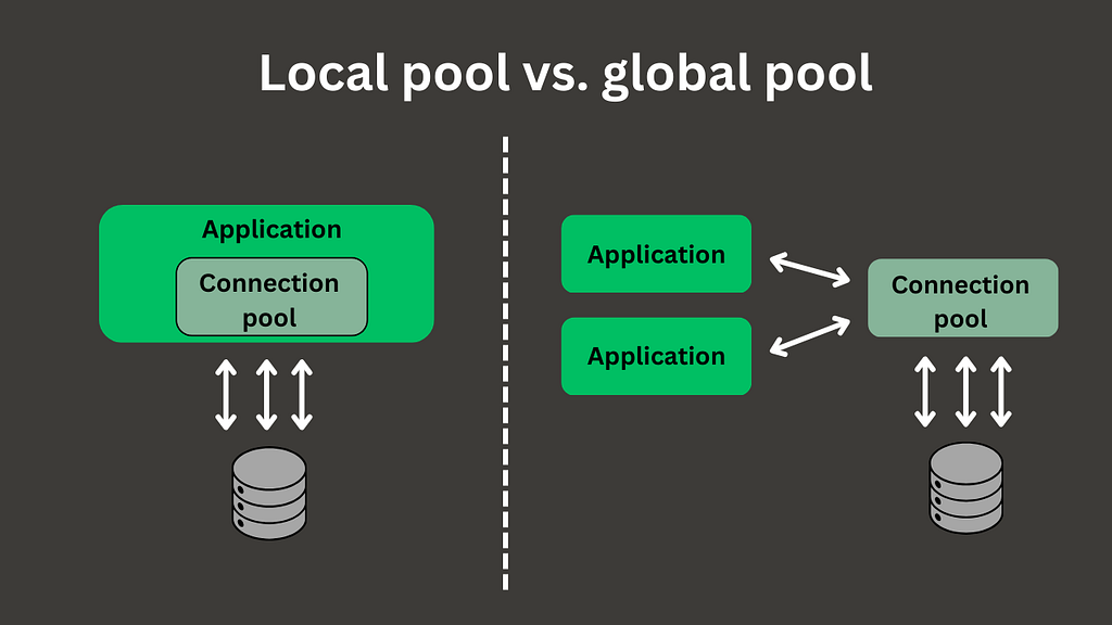
One thing that should definitely be considered is the use of connection pooling. A connection pool is a component that acts as a cache for open database connections, allowing them to be reused. Opening a new connection for every request can lead to a significant increase in time for operation execution. That’s because there is a cost associated with the underlying opening/closing of the connection.
When using a connection pool, you have two options: implement it at the application level or as a standalone infrastructure component. The first option is usually chosen when you have only one application connecting to a dedicated database. The second option is appropriate when multiple clients cannot share their connections from a local connection pool, requiring you to manage connection pooling separately.
Compression
As data grows, it requires more and more storage. Not only that, but a database system can become I/O-bound, potentially resulting in a bottleneck.
Many databases support lossless compression algorithms out of the box. The expected benefit is a reduced size of data that needs to be written and read, allowing faster access. The downside is the additional CPU cycles required to compress and decompress the data. However, in most cases, the CPU is fast enough that we still notice a performance speedup.
Caching
Caching is the process of utilizing pre-saved data in fast-access storage to reduce the computation and time needed to fetch data from the main storage. A fast-access storage component is called a cache, and at the software level, it usually takes the form of in-memory storage, such as Redis, Memcached, KeyDB, etc.
There are several strategies to implement caching. As you will see, each strategy has a trade-off between write speed, data inconsistency, and architecture resilience.
Cache-aside
A cache-aside strategy is the most simple pattern to use for caching. In this setup, a cache provider is located next to the primary data storage. Any time an application needs to fetch the data, it will go to the cache and read it from there. If there is a cache miss, then the application will read from the database and rehydrate the cache.

The problem with this strategy it’s a cache invalidation: once a record is stored in the cache, it’s no longer reupdated. Since all orchestration is done by the application, the responsibility for cache invalidation is on the developer’s shoulders.
Read-through
In a read-through cache strategy, a cache is sitting in the middle between the application and the database. It may be a part of the database or as a standalone provider, such as Redis. In any case, a read request will always go through the cache level: if there is a cache hit, then data is immediately returned; otherwise, the cache component will go to the database, replicate the record in cache storage, and return the requested resource.
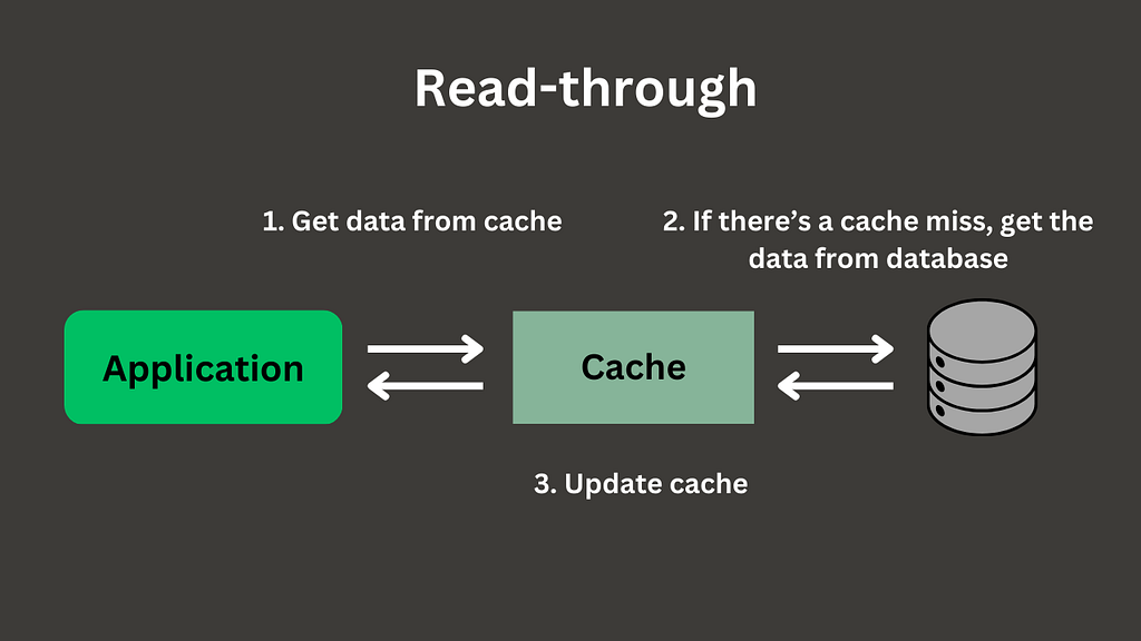
The drawback of this strategy is the same as that of a read-aside strategy: having to update the cache. The advantage, compared to the previous strategy, is that reading operations go to the single entry point in the form of a cache component, and it takes care of itself for cache miss.
Write-around
A write-around strategy is a primary strategy on how you add new data with configured cache-aside or read-through caching setups. In this strategy, new information is written directly to the database and read from the cache. The pros and cons are the same as the chosen cache-read strategy. This design is better suited for frequent data reads and rare data updates.

Write-through
Instead of writing and reading separately, a write-through strategy combines these two operations. When new data arrives to the application, the application issues a new write request directly to the cache component. A cache then stores this copy of data and immediately requests a write operation to the database.

Direct writing to the cache can introduce more latency compared to direct writing to the database.
Another downside of this strategy is the single point of failure. When the cache is down, the application needs to be reconfigured to write to the database. As a potential solution to overcome this problem is to spin multiple cache nodes.
On the contrary, the benefit of a write-through setup is the removed data inconsistency and lack of the need to warm up the cache to ensure all up-to-date data will be present in that component.
Write-back
A write-back caching strategy is similar to the previous one except for one difference: it writes to the database once in a while instead of immediately writing.

This results in improved time for write delay as the number of network roundtrips between the cache and the database can be dramatically decreased. It will be the best choice for applications with a write-heavy workload.
But it also means that the data will have an eventual consistency. And as with write-through there is a chance for data loss in case of cache system failure.
As was shown, there is no silver bullet approach to implementing caching; every strategy has its own drawbacks. You choose what’s suitable for your concrete use case. However, you can also tune these caching strategies if needed. For example, you may add a custom algorithm to the write-around strategy to improve the data consistency characteristic. Or, with cache-aside or read-through, you can warm up the cache by issuing common queries.

Partitioning
Database partitioning is a technique that splits data into chunks so that all operations are performed directly on the fragments rather than on the entire data set, which speeds up the overall performance of the system. Generally, it falls into two main categories: vertical and horizontal partitioning.
You may have already heard about vertical and horizontal scalability. Vertical scaling involves adding more resources to a single machine, such as increasing RAM, CPU cores, or storage space. Whereas, horizontal scaling involves using multiple machines to improve overall computation ability. In terms of partitioning, the concept is similar.
As a rule of thumb, you don’t need partitioning when you have a small table, and your data ingesting pace isn’t going to be high.
Vertical partitioning
Vertical partitioning is a type of partitioning that involves splitting a table by columns into several tables.

In the classical table, you store all data together, but in the vertical partitioned one, you can store ‘hot’ columns in the dedicated table and the rest of the columns in the main table.
The benefit of such a partition is that it reduces the amount of data per row that needs to be scanned. When you need to fetch only the columns stored in some partition, you query it directly, which can give a noticeable performance gain over querying specific columns in a table with many attributes.
Vertical partitioning also gives the ability to store different partitions on different machines: partitions with frequently updated columns could be stored in more performant, high-throughput database servers, and partitions with infrequent update rates or fragments with static fields can be kept on less performant instances.
The disadvantage of vertical partitioning, however, is that in the case of a full data request, it requires additional joins across partitions in comparison with a single table request that stores all the data together. It’s worth noting that overall maintenance also increases, such as dealing with indexes and constraints over partitions.
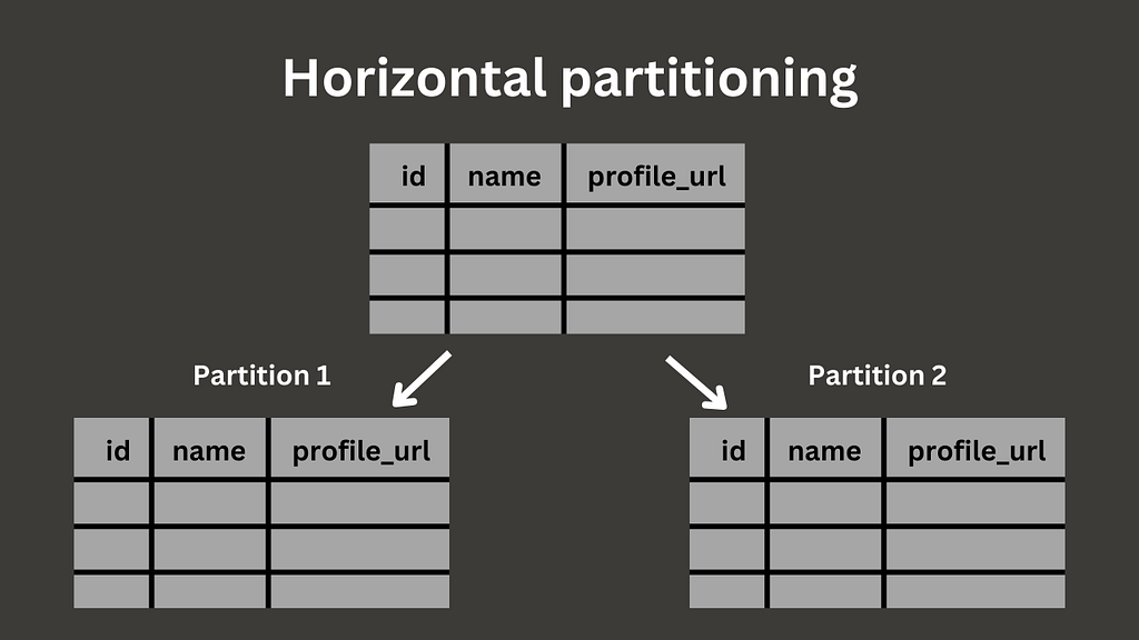
Horizontal partitioning
Horizontal partitioning is a type of partitioning that involves splitting a table by rows into several smaller tables. These subtables have an identical structure to the original table.
Horizontal partitioning is useful for several reasons. One of them is to improve query performance. If you have a large data table or expect it to be so, is wise to consider utilizing partitioning benefits. Instead of going row by row to scan a table, you only need to find a needed partition range that, as in result, can dramatically decrease query time.
A prime example of horizontal partitioning is when working with time-bound (time series) data. By partitioning data based on specific time ranges, you can quickly locate the required time bucket. Another example is partitioning rows by columns with specific value ranges, such as enumerations, allowing you to query only the subset of data that matches the value you’re interested in.
You may ask why you should not just use an index. This is because with a large amount of data, an index scan becomes less beneficial, and there is a higher maintenance overhead, for example, when you need to defragment deleted values.
Another benefit of horizontal partitioning is the ease of data management. If we want to control partitioned data independently, partitioning facilitates that. For instance, if we want to delete records for a specific month and year, we can partition the data by time and treat the resulting chunks as standalone sets. This approach ensures that when we delete a particular chunk, all associated data is removed as well. It is also much faster and more resource-efficient than deleting a set of rows individually.
Managing partitions must done carefully. Picking the wrong partition attributes can lead to uneven data distribution, causing performance bottlenecks. Or the opposite, if you over-partition your dataset, it takes away all the advantages due to query planning overhead.
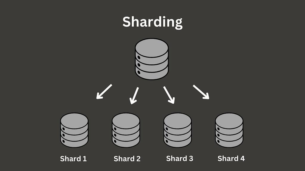
Sharding
Sharding is a technique of storing a large dataset on multiple machines called shards. The principle of splitting the data remains the same as in the previous chapter. Typically, sharding is done using horizontal partitioning.
What benefits does this bring? One of the most obvious is that you can now store data closer to your customers. For example, if we shard a database table by location, we can store different shards in different regions, thereby improving latency. Another advantage of sharding is that the database load can be distributed across different hardware, enhancing overall system performance.
That may sound like a universal solution to dealing with database performance, doesn’t it? However, as you may know, everything comes with a cost, and sharding is no exception. The challenge lies in choosing a shard key that will uniquely identify a single partition. If you fail with this task, then you will have to scan several shards to find the needed information, thus removing the main point of sharding. Data backup is also starting to get complicated: instead of backing up a single table, you now have to consider several shards. The same goes for replication, synchronization, and overall operation complexity. So, the decision to implement sharding should be made cautiously, with all benefits and drawbacks in mind.
Replication
Database replication is a technique that involves creating copies of databases across different servers. You can think about it as a file backup process that is used to ensure data will not be lost when the main source is damaged or cannot be accessed.
The main benefits of database replication include reducing the workload on the data storage layer, providing fault tolerance in case of a crash, enabling scaling by allowing reading from and writing to multiple database instances, and improving user experience by locating a database replica closer to the end user.
When it comes to implementing replication, there are two main strategies: master-slave and multi-master.
Master-slave replication
Master-slave replication, sometimes called single-leader, primary-secondary, or active-passive, is a type of replication where there is only one primary node that is in charge of modifying data and multiple secondary nodes that serve read requests. Every node in this setup holds the same copy of data so that the read commands can be delegated to one of them.

As we have more instances of database we can easily scale read operations. But what about the write operations? Commands like INSERT, UPDATE, DELETE become tricky because there is only one entry that accepts it. Also, there is additional time for data synchronization between the primary and secondary nodes.
And what if the main node goes down? Well, there are several mechanisms to deal with it, but the common one is that the system tries to take one of the active replicas and make it a master replica.
As you can see, this architectural strategy is more suitable when there is no expectation of high write throughput, as the master node becomes the bottleneck of such a setup.
Multi-master replication
Multi-master replication, sometimes called multi-leader, is a type of replication where there are multiple primary nodes that handle read and write requests. It is typically used when shortcomings of the previous strategy are critical.

Each node responsible for write and read operations can optionally have a set of nodes handling only read operations, thus forming multiple local subclusters and combining master-slave and multi-master strategies together.

By providing multiple nodes that can handle write operations, this setup eliminates the potential single point of failure in case the master node goes down. In addition to it, it distributes write operations, so scaling those can now be possible.
The drawback, however, is that it is hard to synchronize modified data. Imagine a case where the same piece of data is modified on multiple nodes. It’s also worth noting that the more nodes you have, the more time it takes to synchronize them. So, this setup is definitely complex to configure.
Conclusion
In the final part, I want to remind you of the two-step process for enhancing database performance.
First of all, you need to understand what exactly causes a performance decrease. It may be a particular operation such as a heavy join, a set of operations on an increasingly large dataset, network latency, or a redundant big payload.
Once you’ve pinpointed the issue, the next step is selecting the appropriate solution. As we’ve discussed, different strategies address different aspects of database performance, whether it’s query optimization, indexing, denormalization, configuration tuning, caching, partitioning, sharding, or replication.
While choosing a solution, consider not only the benefits but also the potential drawbacks of each strategy. Some methods might improve speed at the cost of increased complexity or resource consumption. Evaluate your chosen approach’s impact by measuring performance before and after implementation. Having the right balance is key to achieving sustainable, long-term improvements for your database.
Thank you for reading this article!
Any questions or suggestions? Feel free to write a comment.
I’d also be happy if you followed me and gave this article a few claps! 😊
Check out some of my latest articles here:
In Search of Improving Database Performance: A Comprehensive Guide with 8 Key Strategies was originally published in Level Up Coding on Medium, where people are continuing the conversation by highlighting and responding to this story.
This content originally appeared on Level Up Coding - Medium and was authored by Pavlo Kolodka
Pavlo Kolodka | Sciencx (2024-09-02T01:17:18+00:00) In Search of Improving Database Performance: A Comprehensive Guide with 8 Key Strategies. Retrieved from https://www.scien.cx/2024/09/02/in-search-of-improving-database-performance-a-comprehensive-guide-with-8-key-strategies/
Please log in to upload a file.
There are no updates yet.
Click the Upload button above to add an update.