This content originally appeared on HackerNoon and was authored by Restructure
:::info Authors:
(1) Oleksandr Kuznetsov, Proxima Labs, 1501 Larkin Street, suite 300, San Francisco, USA and Department of Political Sciences, Communication and International Relations, University of Macerata, Via Crescimbeni, 30/32, 62100 Macerata, Italy (kuznetsov@karazin.ua);
(2) Dzianis Kanonik, Proxima Labs, 1501 Larkin Street, suite 300, San Francisco, USA;
(3) Alex Rusnak, Proxima Labs, 1501 Larkin Street, suite 300, San Francisco, USA (alex@proxima.one);
(4) Anton Yezhov, Proxima Labs, 1501 Larkin Street, suite 300, San Francisco, USA;
(5) Oleksandr Domin, Proxima Labs, 1501 Larkin Street, suite 300, San Francisco, USA.
:::
Table of Links
1.1. The Blockchain Paradigm and the Challenge of Scalability
1.3. Our contribution and 1.4. Article structure
2. Conceptualizing the Problem
3. Our Idea for Optimizing Trees in Blockchain
4. Efficiency of adaptive Merkle trees
5. Algorithm for Merkle Tree Restructuring
6.2. Example 1.1: Binary Tree Restructuring Through Leaf Node Swapping
6.3. Example 2.1: Restructuring a Non-Binary Tree by Adding a Single Leaf
6.4. Example 2.2: Restructuring a Non-Binary Tree Through Leaf Pair Swapping
6.5. Example 2.3: Restructuring a Patricia-Merkle Tree Fragment Through Leaf Pair Swapping
7. Path Encoding in the Adaptive Merkle Tree
8.2. Technology and Advantages
9.2. Comparison with Existing Solutions
6. Examples of Merkle Tree Restructuring Algorithm Execution
To illustrate the algorithm's application, let's consider the case of a binary tree where one new leaf is added at each iteration. Initially, we form a list of alternatives for all leaves in the previous tree configuration. Each leaf can be transformed into an intermediate node with two child nodes: one from the previous configuration and one new (added) leaf.
6.1 Example 1: Restructuring a Binary Tree by Adding One Leaf
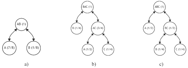
Suppose we have a small binary ( m = 2 ) balanced tree consisting of two nodes A and B, with probabilities 7/8 and 1/8, respectively (see Fig. 11, a).
\
\ Assume that at the next moment, a new leaf C is created with probabilities now equal to:
\ A (1/2), B (1/4), C (1/4).
\ Our goal is to add this new leaf C in such a way as to minimize the average discrepancy (1). Here and subsequently, we assume that all branches from the previous tree configuration are available for addition.
\ 6.1.1. First Iteration
\ On the first iteration, we have two alternatives for adding the new leaf to the previous tree configuration. These alternatives are presented in Fig. 11 and Table 1.
\ The first alternative (see Fig. 11, b) corresponds to adding node C (1/4) to the branch with node A (1/2). As we can see from Table 1, this increases the discrepancy . The second alternative (see Fig. 11, c) is more preferable as the discrepancy (1) here is significantly lower (equals zero), i.e., node C (1/4) should be added to the branch with node B (1/4).
\

\ Therefore, by the criterion of minimizing (1), we select the second alternative, i.e., the tree presented in Fig. 11, c. From the perspective of path length, this option is optimal as its average discrepancy (1) equals zero. Essentially, this indicates that we have achieved an ideal structure for this probability distribution.
\ Continuing from the initial iteration of the Merkle Tree restructuring algorithm, let us delve into subsequent iterations to further elucidate the process and its outcomes.
\ 6.1.2. Second Iteration
\ Let us assume that in the second iteration, a new leaf, D, is introduced, leading to a new probability distribution among the leaves:
\ A (1/2), B (1/8), C (1/4), and D (1/8).
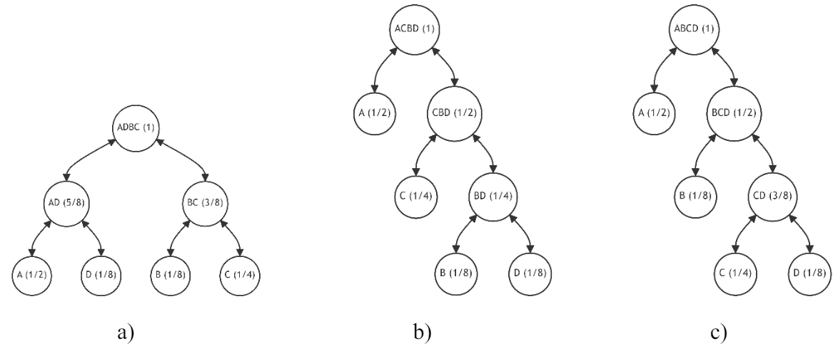
\ Building upon the tree's previous state (refer to Fig. 11, c), we are presented with three distinct restructuring alternatives (illustrated in Fig. 12):
\ a) Integrating the new node D (1/8) into the branch containing node A (1/2);
\ b) Integrating the new node D (1/8) into the branch containing node B (1/8);
\ c) Integrating the new node D (1/8) into the branch containing node C (1/4).
\ For each alternative, we calculate the average discrepancy, as detailed in Table 2. The most favorable alternative, marked by a zero discrepancy, is highlighted in the table.
\
\
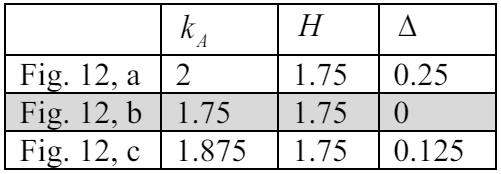
\ Accordingly, the second alternative (see Fig. 12, b) emerges as the most preferable, characterized by a zero average discrepancy, indicating an optimal restructuring choice under the given criteria.
\ 6.1.3. Third Iteration
\ Advancing to the third iteration, let's hypothesize the addition of another new leaf, E, resulting in the following probability distribution:
\ A (1/2), B (1/8), C (1/8), D (1/8), E (1/8).
\ The tree structure that achieves a zero discrepancy, indicative of an optimal configuration minimizing the average path length, is depicted in Fig. 13.
\
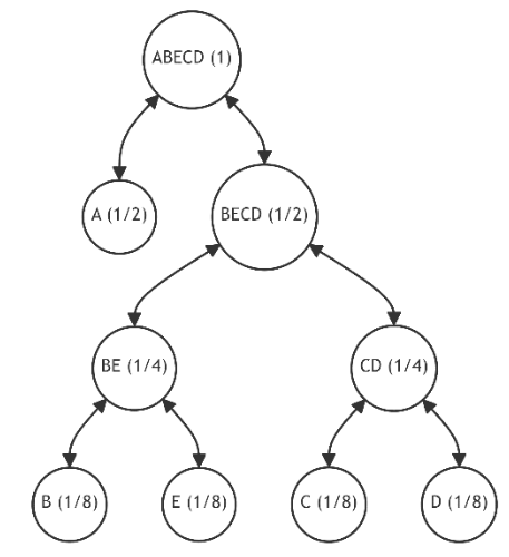
\ Achieving a zero discrepancy signifies that we have attained an optimal tree structure, effectively minimizing the average path length.
\ 6.1.4. Fourth Iteration
\ During the fourth iteration, we face the task of incorporating an additional leaf, resulting in a new probability distribution:
\ A (1/2), B (1/4), C (1/16), D (1/16), E (1/16), F (1/16).
\

\
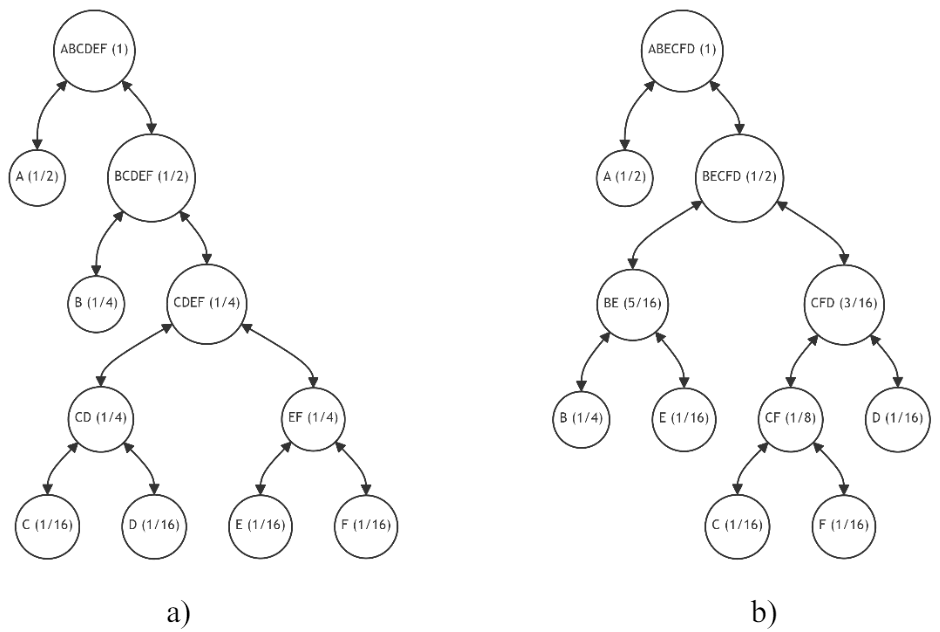
\ Utilizing the tree from Figure 13, we identify five potential alternatives (refer to Table 3), none of which lead to the desired configuration seen in Figure 14.a.
\ In Table 3, we present a comparison of all possible alternatives based on the average discrepancy value (1). It becomes evident that the last three alternatives are equivalent in terms of their potential outcomes, and thus, the choice of restructuring can be made arbitrarily. We decide to employ a lexicographical ordering rule, selecting alternative "C" as illustrated in Figure 14.b. Although this new structure is not optimal, it achieves the minimum average discrepancy of 0.125 among all possible restructuring scenarios.
\

\ 6.1.5. Iterations 5-10
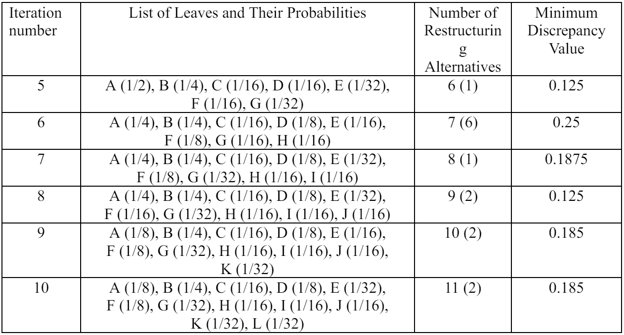
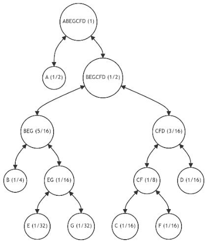
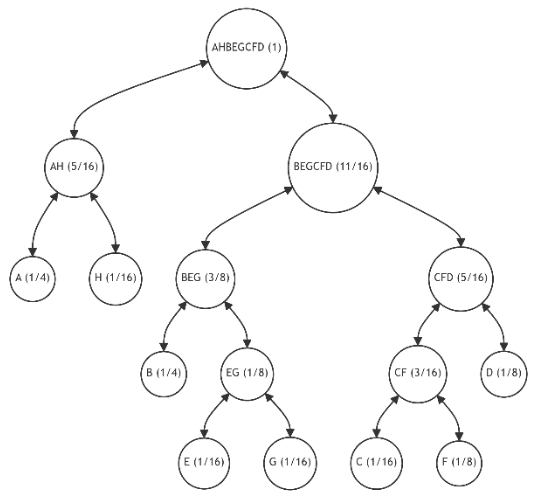
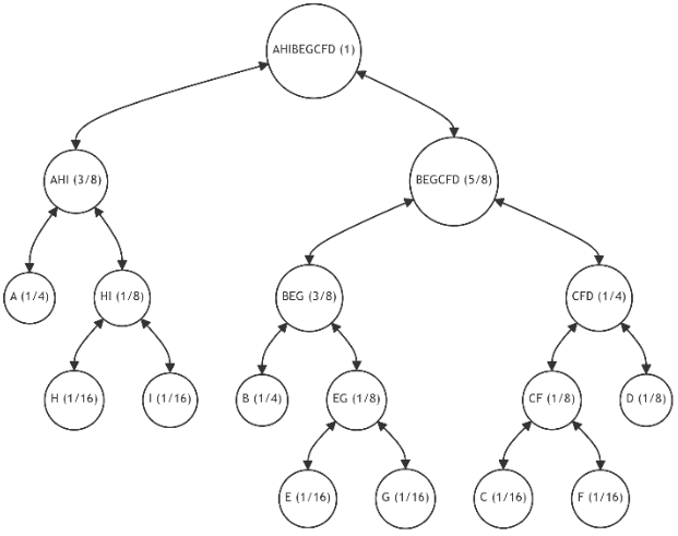
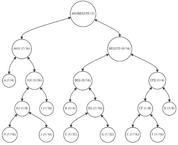
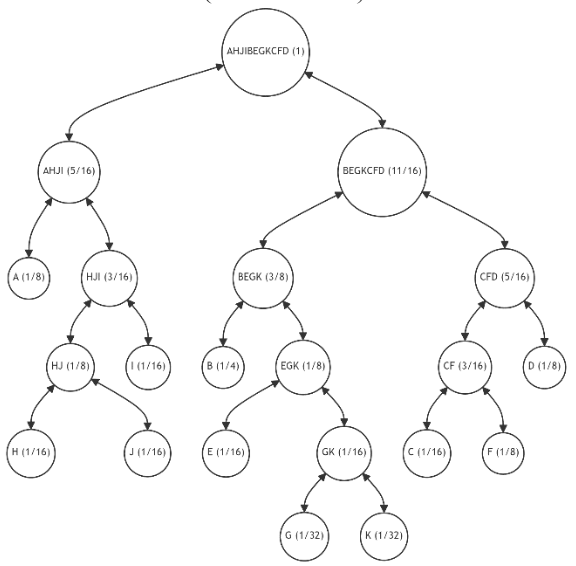
\ For further illustration, let's assume that each subsequent iteration introduces one additional leaf, with the probability distribution for the tree's leaves as specified in Table 4. This table also indicates the number of available restructuring alternatives and (in parentheses) the number of alternatives with the minimum discrepancy value. The last column provides the minimum discrepancy value (11) across all alternatives. Figures 15-20 showcase the restructuring outcomes based on the chosen optimal alternative.
\
\
\
\
\
\
\
\
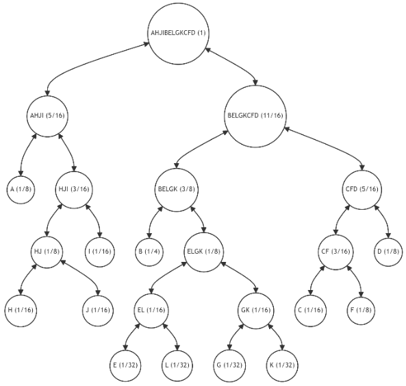
\ The table reveals that, despite an increase in the number of alternatives with each iteration, the number of most preferable restructuring options remains limited. Moreover, despite fluctuations in the probabilities of individual leaves, we consistently approach an optimal tree structure.
\ To further enhance the efficiency of tree restructuring, we propose expanding the algorithm's parameters. This involves forming potential alternatives not just by adding leaves but by considering various scenarios for swapping the positions of leaf pairs. This approach is particularly relevant in blockchain transactions, which typically involve at least two accounts, thus allowing for the repositioning of leaves by exchanging their locations.
\ This expansion of the algorithm's capabilities demonstrates our commitment to optimizing tree structures for improved verification efficiency, paving the way for more dynamic and efficient blockchain architectures.
\
:::info This paper is available on arxiv under CC by 4.0 Deed (Attribution 4.0 International) license.
:::
\
This content originally appeared on HackerNoon and was authored by Restructure
Restructure | Sciencx (2024-09-10T23:30:27+00:00) Examples of Merkle Tree Restructuring Algorithm—Execution and Example 1: Restructuring a Binary. Retrieved from https://www.scien.cx/2024/09/10/examples-of-merkle-tree-restructuring-algorithm-execution-and-example-1-restructuring-a-binary/
Please log in to upload a file.
There are no updates yet.
Click the Upload button above to add an update.
