Want to Decrease Your Model’s Prediction Errors by 20%? Follow This Simple Trick

This content originally appeared on Level Up Coding - Medium and was authored by Philippe Ostiguy, M. Sc.

Make your time series stationary automatically using Python

Time series modeling can be tricky, even for experienced data scientists. You’ve done everything by the book: used state-of-the-art deep learning models, performed feature engineering, normalized your data, and optimized hyperparameters. Yet, your model’s performance still falls short. If this your case, this simple change may help you.

What if there was one key step you might be overlooking? A step that could potentially improve your model’s performance by 20%? In a previous article on custom validation metric for stock forecasting, we encountered a critical aspect of time series preprocessing: making your data stationary.

But here’s the catch — this crucial step isn’t always straightforward. Different variables and time series can have various shapes — some are linear, while others might be exponential. This means that the transformation required isn’t always a simple first differentiation.

You might be wondering why it’s important and do we automate it? That’s exactly what we’ll discuss in this article. Here’s a quick summary of what will be covered:

• Importance of making your data stationary— We’ll explore why our time series and exogenous variables must be stationary before training a model. We’ll show a non-stationary example where the model failed to generalize.
• Implementation guide — We’ll provide detailed step-by-step instructions to automatically make both your time series and exogenous variables stationary using Python. We’ll walk you through the necessary methods and tests to ensure that your data are ready in your pipeline.

Why Does Your Data Need to Be Stationary?

First, what is a stationary time series? It’s a time series in which statistical properties, such as mean, variance and covariance, remain constant over time. A picture is worth a thousand words :

import yfinance as yf
import matplotlib.pyplot as plt
spy = yf.Ticker("SPY")
data = spy.history(period="10y")

plt.figure(figsize=(10, 5))
plt.plot(data.index, data['Close'], label='SPY Close Price')
plt.title('SPY Closing Prices (Last 10 Years)')
plt.xlabel('Date')
plt.ylabel('Close Price')
plt.legend()
plt.show()

monthly_returns = data['Close'].pct_change().dropna()

plt.figure(figsize=(10, 5))
plt.plot(monthly_returns.index, monthly_returns, label='SPY Monthly Return')
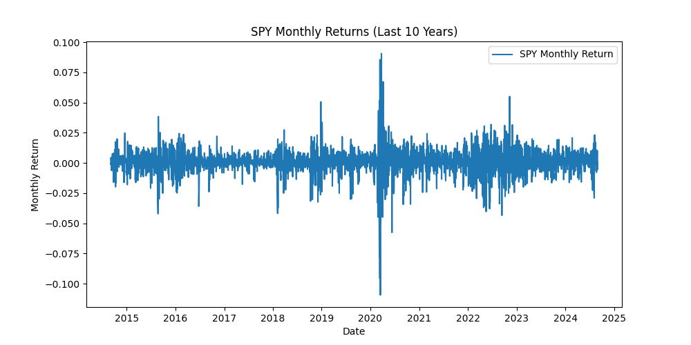
plt.title('SPY Monthly Returns (Last 10 Years)')
plt.xlabel('Date')
plt.ylabel('Monthly Return')
plt.legend()
plt.show()

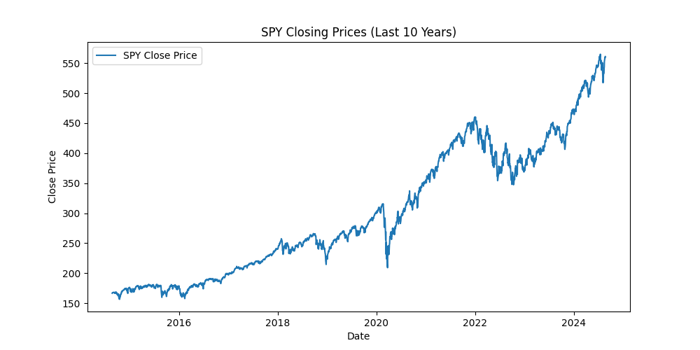
In the first example, the mean isn’t constant over time, showing a clear trend in the SPY price. This indicates that the series is non-stationary.

In the second example, the mean stay around 0, and the variance remains mostly stable, except during the 2020 pandemic when volatility spiked. This series is at least weakly stationary.

It’s easy to validate with the Augmented Dickey–Fuller test.

from statsmodels.tsa.stattools import adfuller
def get_p_value(series):
    result = adfuller(series, autolag='AIC')
    return result[1]

price_p_value = get_p_value(data['Close'])

returns_p_value = get_p_value(monthly_returns)

print(f"\np-value for stock price: {price_p_value}")
print(f"p-value for monthly returns: {returns_p_value}")

At a 95% level confidence, having we can confirm that the stock price is not stationary and the monthly returns are stationary.

Ok. We understand what a stationary time series is, but why should we care? Shouldn’t foundation models and Transformer-based models handle non-stationary time series automatically? Not quite…

We’ll use PatchTST, a state-of-the-art Transformer-based model. We’ll use the implementation provided by NeuralForecast. We’ll train and test two models using monthly SPY (S&P 500 ETF) data. Both models will have the same:

1. Train-test split ratio
2. Hyperparameters
3. No exogenous variables
4. Single time series
5. Forecasting horizon of 1 step ahead

The only difference between the models will be the data type. That’s it!

1. First model: Non-stationary data (SPY price)
2. Second model: Stationary data (SPY monthly returns)

For each model, we’ll forecast one step ahead for every data point in the test set for both the SPY price and SPY monthly returns.

from neuralforecast.models import PatchTST
from neuralforecast import NeuralForecast
import yfinance as yf
import matplotlib.pyplot as plt
import pandas as pd
import numpy as np

spy = yf.Ticker("SPY")
spy_data = spy.history(start="2010-01-01", end="2023-12-31")
spy_data = spy_data.resample('M').last().reset_index()
spy_data.columns = ['ds', 'y'] + list(spy_data.columns[2:])
spy_data = spy_data[['ds', 'y']]
spy_data['unique_id'] = 'SPY'
spy_data['returns'] = spy_data['y'].pct_change()
spy_data = spy_data.dropna()

train_size = int(len(spy_data) * 0.8)
train_data = spy_data[:train_size]
test_data = spy_data[train_size:]

model = PatchTST(
    h=1,
    input_size=24,
    scaler_type='standard',
    max_steps=100
)

nf = NeuralForecast(
    models=[model],
    freq='M'
)

nf.fit(df=train_data)

test_size = len(test_data)
y_hat_test_price = pd.DataFrame()
current_train_data = train_data.copy()

future_predict = pd.DataFrame({'ds': [test_data['ds'].iloc[0]], 'unique_id': ['SPY']})

y_hat_price = nf.predict(current_train_data, futr_df=future_predict)
y_hat_test_price = pd.concat([y_hat_test_price, y_hat_price.iloc[[-1]]])

for i in range(test_size - 1):
    combined_data = pd.concat([current_train_data, test_data.iloc[[i]]])
    future_predict['ds'] = test_data['ds'].iloc[i + 1]
    y_hat_price = nf.predict(combined_data, futr_df=future_predict)
    y_hat_test_price = pd.concat([y_hat_test_price, y_hat_price.iloc[[-1]]])
    current_train_data = combined_data

predictions_prices = y_hat_test_price['PatchTST'].values
true_values = test_data['y'].values

mse = np.mean((predictions_prices - true_values)**2)
rmse = np.sqrt(mse)
mae = np.mean(np.abs(predictions_prices - true_values))

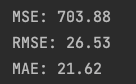
print(f"MSE: {mse:.2f}")
print(f"RMSE: {rmse:.2f}")
print(f"MAE: {mae:.2f}")

plt.figure(figsize=(12, 6))
plt.plot(train_data['ds'], train_data['y'], label='Training Data', color='blue')
plt.plot(test_data['ds'], true_values, label='True Values', color='green')
plt.plot(test_data['ds'], predictions_prices, label='Predictions', color='red')
plt.legend()
plt.title('SPY Stepwise Forecast using PatchTST')
plt.xlabel('Date')
plt.ylabel('SPY Price')
plt.show()

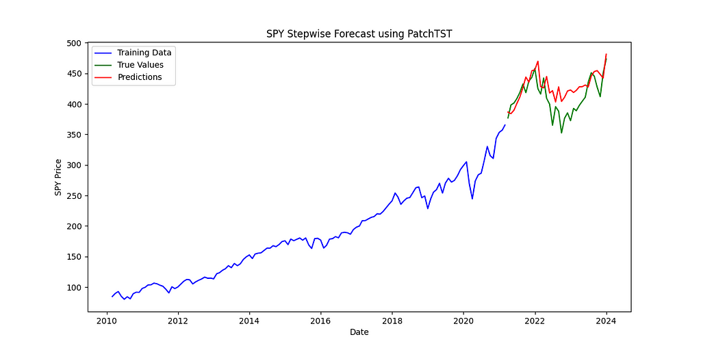
Looking at the chart, the accuracy of the model seems reasonable. Now, let’s examine the forecast for the stationary data (monthly returns).

model = PatchTST(
    h=1,
    input_size=24,
    scaler_type='standard',
    max_steps=100
)

nf = NeuralForecast(
    models=[model],
    freq='M'
)

nf.fit(df=train_data[['ds', 'returns', 'unique_id']].rename(columns={'returns': 'y'}))

y_hat_test_ret = pd.DataFrame()
current_train_data = train_data[['ds', 'returns', 'unique_id']].rename(columns={'returns': 'y'}).copy()

future_predict = pd.DataFrame({'ds': [test_data['ds'].iloc[0]], 'unique_id': ['SPY']})

y_hat_ret = nf.predict(current_train_data, futr_df=future_predict)
y_hat_test_ret = pd.concat([y_hat_test_ret, y_hat_ret.iloc[[-1]]])

for i in range(test_size - 1):
    combined_data = pd.concat([current_train_data, test_data[['ds', 'returns', 'unique_id']].rename(columns={'returns': 'y'}).iloc[[i]]])
    future_predict['ds'] = test_data['ds'].iloc[i + 1]
    y_hat_ret = nf.predict(combined_data, futr_df=future_predict)
    y_hat_test_ret = pd.concat([y_hat_test_ret, y_hat_ret.iloc[[-1]]])
    current_train_data = combined_data

predicted_returns = y_hat_test_ret['PatchTST'].values
true_returns = test_data['returns'].values

predicted_prices_ret = []
for i, ret in enumerate(predicted_returns):
    if i == 0:
        last_true_price = train_data['y'].iloc[-1]
    else:
        last_true_price = test_data['y'].iloc[i-1]
    predicted_prices_ret.append(last_true_price * (1 + ret))

mse = np.mean((np.array(predicted_prices_ret) - true_values)**2)
rmse = np.sqrt(mse)
mae = np.mean(np.abs(np.array(predicted_prices_ret) - true_values))

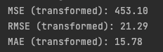
print(f"MSE (transformed): {mse:.2f}")
print(f"RMSE (transformed): {rmse:.2f}")
print(f"MAE (transformed): {mae:.2f}")

plt.figure(figsize=(12, 6))
plt.plot(train_data['ds'], train_data['y'], label='Training Data', color='blue')
plt.plot(test_data['ds'], true_values, label='True Prices', color='green')
plt.plot(test_data['ds'], predicted_prices_ret, label='Predicted Prices', color='red')
plt.legend()
plt.title('SPY Stepwise Forecast using PatchTST (Prices)')
plt.xlabel('Date')
plt.ylabel('SPY Price')
plt.show()

We forecast the monthly returns using the model, then convert these back to prices. This allows us to calculate prediction errors using prices and compare the actual prices to the forecasted prices in a plot.

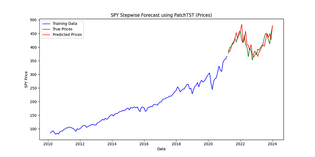
There’s a big difference between two identical models when we change only the input data. This holds true even for a state-of-the-art model like PatchTST, which is designed to handle unfamiliar data effectively:

• Non-stationary data (stock prices)
• Stationary data (monthly returns)

This change alone improved the model’s performance:

• RMSE went from 26.53 to 21.29 (20% decrease)
• MSE went from 703.88 to 453.10 (36% decrease)

Why the difference? The test data had new record-high prices that the model hadn’t seen during training. The model was used to predict data that deviate substantially from the data it was trained on. This made it hard for the model to generalize well. In contrast, the model produced better forecasts for stock returns on unseen data. Why? Because monthly stock returns remain within a familiar range, presenting little or no data that the model hadn’t been exposed to during training.

This shows why it’s important to use stationary data in time series analysis. By making this one change, we increase the model robustness and its ability to generalize better on unseen data. This is especially important for financial and economic data. Think about things like GDP or stock prices — they tend to grow exponentially over time. Without making the data stationary, your model might have to predict situations it’s never seen before during training.

Ok. We understand the importance of making data stationary, but is there a way to automate this process? Can we avoid transforming each feature individually? Yes, there is.

We will focus on transformations for financial and economic time series. However, the same principles apply to other types of time series. We’ll cover the most common transformations, but keep in mind that there are other useful methods available, such as the Box-Cox transformation.

First, we’ll apply three transformations and replace any NaN or infinite values with the previous valid value:

• First differentiation
• Percentage change
• Logarithmic transformation

spy_data['first_diff'] = spy_data['y'].diff()
spy_data['pct_change'] = spy_data['y'].pct_change()
spy_data['log'] = np.log(spy_data['y'])
spy_data =spy_data.drop(spy_data.index[0])
spy_data = spy_data.reset_index(drop=True)

def replace_inf_nan(series):
    if np.isnan(series.iloc[0]) or np.isinf(series.iloc[0]):
        series.iloc[0] = 0
    mask = np.isinf(series) | np.isnan(series)
    series = series.copy()
    series[mask] = np.nan
    series = series.ffill()
    return series

columns_to_test =  ['first_diff', 'pct_change','log', 'y']
for col in columns_to_test:
    spy_data[col] = replace_inf_nan(spy_data[col])

has_nan = np.isnan(spy_data[columns_to_test]).any().any()
has_inf = np.isinf(spy_data[columns_to_test]).any().any()

print(f"\nContains NaN: {has_nan}")
print(f"Contains inf: {has_inf}\n")

Next, we’ll plot the original time series along with the three transformed versions.

plt.figure(figsize=(10, 6))
plt.plot(spy_data.index, spy_data['y'])
plt.title('SPY Data - Original Values')
plt.xlabel('Index')
plt.ylabel('Value')
plt.grid(True)
plt.show()

plt.figure(figsize=(10, 6))
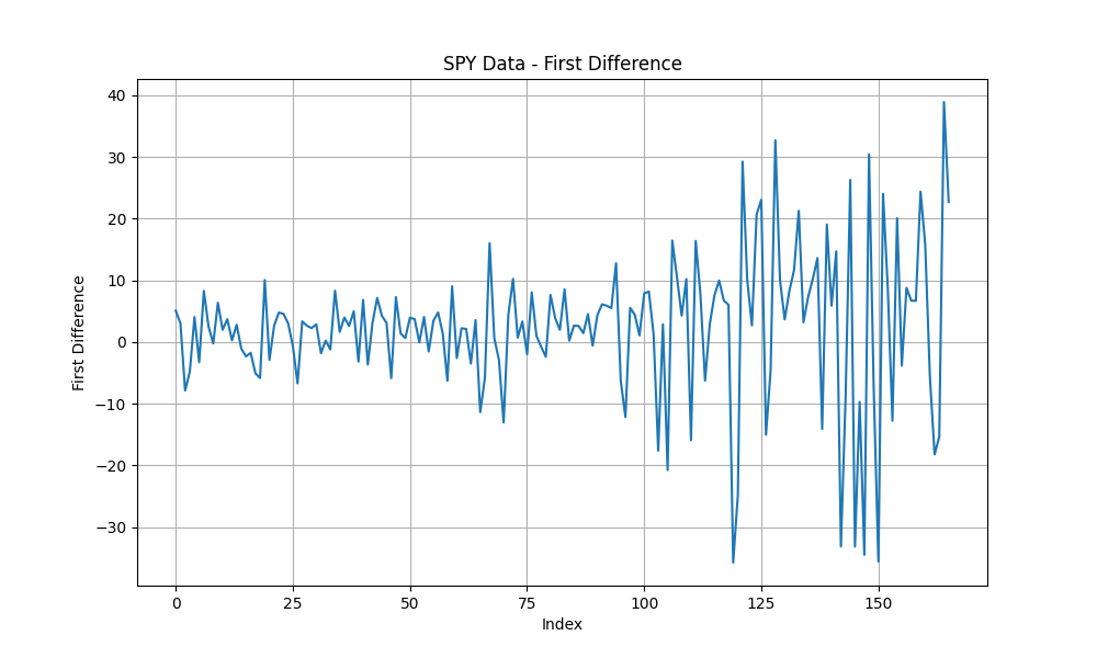
plt.plot(spy_data.index, spy_data['first_diff'])
plt.title('SPY Data - First Difference')
plt.xlabel('Index')
plt.ylabel('First Difference')
plt.grid(True)
plt.show()

plt.figure(figsize=(10, 6))
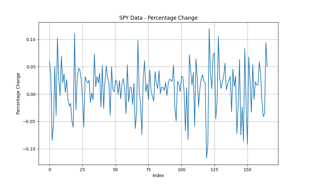
plt.plot(spy_data.index, spy_data['pct_change'])
plt.title('SPY Data - Percentage Change')
plt.xlabel('Index')
plt.ylabel('Percentage Change')
plt.grid(True)
plt.show()

plt.figure(figsize=(10, 6))
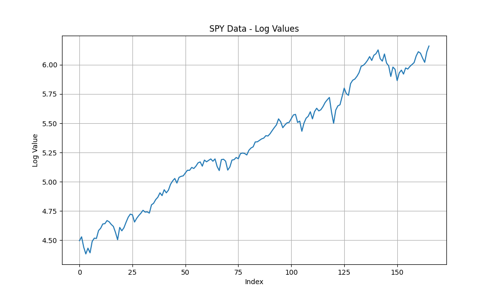
plt.plot(spy_data.index, spy_data['log'])
plt.title('SPY Data - Log Values')
plt.xlabel('Index')
plt.ylabel('Log Value')
plt.grid(True)
plt.show()

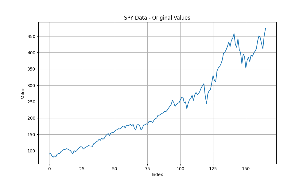
Looking at these plots, we can observe:

• The logarithmic transformation still shows a trend, suggesting the series may be non-stationary.
• The first differentiation exhibits heteroskedasticity — its variance changes over time, increasing in this case. This is expected as the stock market tend to grow exponentially. In other words, when you subtract yesterday’s price from today’s price, the difference tends to be much larger in recent times compared to the difference between prices from dates many years ago. A GARCH model could verify whether the transformation exhibits heteroskedasticity.
• The percentage change appears to have a constant mean and variance over time, potentially indicating stationarity. This is expected, as the percentage change represents the monthly returns, which tend to remain within a range with a constant mean and variance over time.

To validate these observations, let’s apply the Augmented Dickey-Fuller Test.

from statsmodels.tsa.stattools import adfuller
from tabulate import tabulate

results = []

for column in columns_to_test:
    result = adfuller(spy_data[column].dropna())
    results.append([column, result[0], result[1]])

headers = ["Column", "ADF Statistic", "p-value"]
table = tabulate(results, headers=headers, floatfmt=".5f", tablefmt="grid")

print("Augmented Dickey-Fuller Test Results:")
print(table)

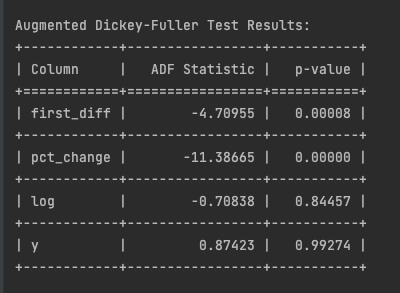
Using a 95% confidence level, the ADF test results reveal important insights about our data transformations:

1. First differentiation and percentage change are stationary (p-values < 0.05).
2. Log transformation and original values (y) remain non-stationary (p-values > 0.05).

With two stationary transformations, how do we choose the ‘right’ one? The key lies in the ADF statistic. A more negative ADF statistic indicates stronger evidence against the null hypothesis of non-stationarity. In this case, the percentage change (-11.38665) shows more compelling evidence of stationarity compared to the first difference (-4.70955). Therefore, we would apply the percentage change transformation to the series. We’ll then repeat this process with the other time series and any exogenous variables.

Conclusion

In conclusion, we discussed the importance of making your time series stationary and how to automate it:

• Making your data stationary can significantly improve your model’s performance. This adjustment alone can reduce prediction errors, such as RMSE by 20% and MSE by 36%, even with state-of-the-art models like PatchTST. This step is crucial for ensuring that models can generalize well.
• To achieve stationarity, apply three key transformations to each of your time series data: first differentiation, percentage change, and logarithmic transformation. These three transformations are typically sufficient for economic or financial time series. However, you can add others, like the Box-Cox transformation, if needed. Next, use the Augmented Dickey-Fuller (ADF) test to check if the p-value is below 5%, which indicates stationarity at a 95% confidence level. If multiple series are considered stationary (p-values under 5%), select the one with the most negative ADF statistic for stronger evidence of stationarity.

On a final note, keep in mind that like any statistical test, the ADF test has its limitations. One of them is that it primarily focuses on detecting changes in the mean, not the variance, which can overlook issues like heteroskedasticity. This is why having multiple possible transformations and pick the ‘best’ one, like we did in this article, can generally mitigates this issue.

In future articles, we’ll apply these transformations to achieve better performance in our models. Stay tuned for more insights!

Liked this article? Show your support!

👏 Clap it up to 50 times

🤝 Send me a LinkedIn connection request to stay in touch

Your support means everything! 🙏

Want to Decrease Your Model’s Prediction Errors by 20%? Follow This Simple Trick was originally published in Level Up Coding on Medium, where people are continuing the conversation by highlighting and responding to this story.

This content originally appeared on Level Up Coding - Medium and was authored by Philippe Ostiguy, M. Sc.

Print Share Comment Cite Upload Translate Updates

APA

Philippe Ostiguy, M. Sc. | Sciencx (2024-09-10T16:44:40+00:00) Want to Decrease Your Model’s Prediction Errors by 20%? Follow This Simple Trick. Retrieved from https://www.scien.cx/2024/09/10/want-to-decrease-your-models-prediction-errors-by-20-follow-this-simple-trick/

MLA

" » Want to Decrease Your Model’s Prediction Errors by 20%? Follow This Simple Trick." Philippe Ostiguy, M. Sc. | Sciencx - Tuesday September 10, 2024, https://www.scien.cx/2024/09/10/want-to-decrease-your-models-prediction-errors-by-20-follow-this-simple-trick/

HARVARD

Philippe Ostiguy, M. Sc. | Sciencx Tuesday September 10, 2024 » Want to Decrease Your Model’s Prediction Errors by 20%? Follow This Simple Trick., viewed ,<https://www.scien.cx/2024/09/10/want-to-decrease-your-models-prediction-errors-by-20-follow-this-simple-trick/>

VANCOUVER

Philippe Ostiguy, M. Sc. | Sciencx - » Want to Decrease Your Model’s Prediction Errors by 20%? Follow This Simple Trick. [Internet]. [Accessed ]. Available from: https://www.scien.cx/2024/09/10/want-to-decrease-your-models-prediction-errors-by-20-follow-this-simple-trick/

CHICAGO

" » Want to Decrease Your Model’s Prediction Errors by 20%? Follow This Simple Trick." Philippe Ostiguy, M. Sc. | Sciencx - Accessed . https://www.scien.cx/2024/09/10/want-to-decrease-your-models-prediction-errors-by-20-follow-this-simple-trick/

IEEE

" » Want to Decrease Your Model’s Prediction Errors by 20%? Follow This Simple Trick." Philippe Ostiguy, M. Sc. | Sciencx [Online]. Available: https://www.scien.cx/2024/09/10/want-to-decrease-your-models-prediction-errors-by-20-follow-this-simple-trick/. [Accessed: ]

rf:citation

» Want to Decrease Your Model’s Prediction Errors by 20%? Follow This Simple Trick | Philippe Ostiguy, M. Sc. | Sciencx | https://www.scien.cx/2024/09/10/want-to-decrease-your-models-prediction-errors-by-20-follow-this-simple-trick/ |

Please log in to upload a file.

There are no updates yet.
Click the Upload button above to add an update.

You must be logged in to translate posts. Please log in or register.