
This content originally appeared on Level Up Coding - Medium and was authored by Philippe Ostiguy, M. Sc.
Get Free, and Reliable Financial Market Data — Machine Learning-Ready
Automate your data collection using Python for seamless stock market forecasting

Ever tried to build a machine learning model for stock forecasting, only to hit a wall when it comes to finding good data? You’re not alone. Getting reliable economic and financial market data without spending a fortune can be tough, and there are plenty of unreliable sources out there.
Here’s the thing: in machine learning, your data is your foundation.It’s better to have a simpler model with quality data than a state-of-the-art model trained on unreliable data.
With very little Python skills only, you can grab all the free, trustworthy data you need to train your model for stock forecasting. I’ll show you how to automatically collect daily data and prepare it for immediate use in your machine learning models for stock forecasting, saving you time and money while ensuring quality.
If you’ve read my earlier piece on getting free financial news headlines, you’ll know I’m all about making good financial headlines accessible. This time, we’re focusing on financial and economic data. And once you’ve got your solid data? Check out my article on using a custom validation loss to improve your deep learning model — it’s a great next step!
Here’s a quick summary of what will be covered:
- Obtaining free and reliable daily economic and financial market data — We’ll demonstrate how to automatically gather all the reliable data you need for your stock market forecasting models. You’ll also have the possibility to customize date ranges for your queries.
- Quick data preparation for your models — We’ll walk you through the process of transforming your collected data into a format ready for immediate use in your machine learning models. As a brief illustration, we’ll use our acquired data to train a transformer-based model from NeuralForecast
Where to get those free and reliable data?
We’ll be using data from the Federal Reserve Economic Data (FRED) St. Louis API. It’s highly reliable due to its official government source, regular updates, and aggregation of information from multiple authoritative institutions. This makes FRED an excellent choice for accurate, trustworthy data in stock forecasting models.
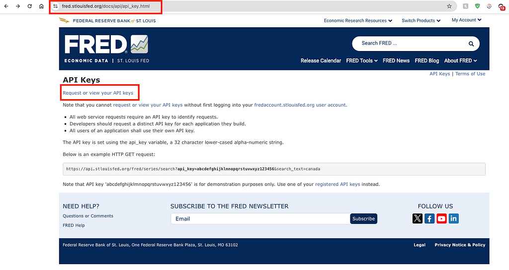
The first step to make API requests to the FRED API is to obtain your free API key here: https://fred.stlouisfed.org/docs/api/api_key.html
1. Request an API key
2. Sign in or create a new account
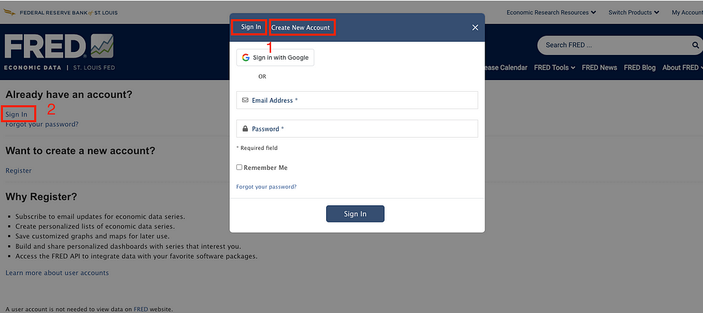
Press the ‘Sign In’ button again (as shown in step 2 of the image above).
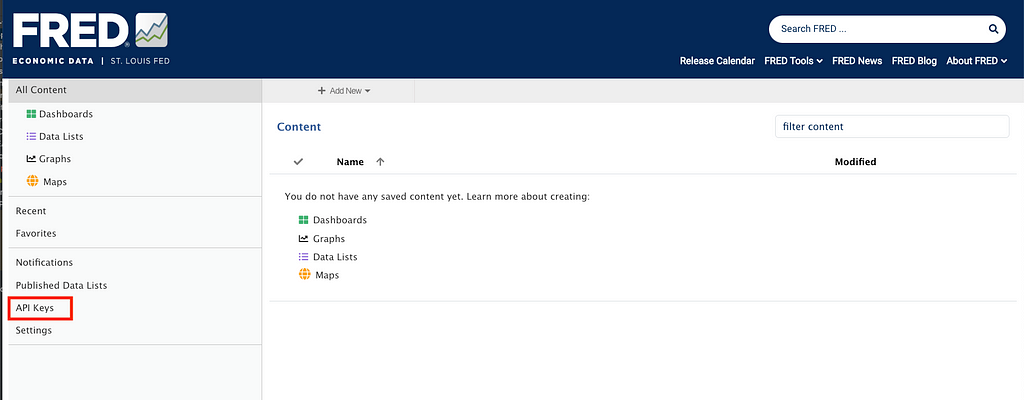
3. Go to the link to request your API key
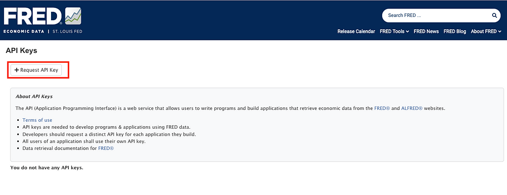
4. Read and agree to the St. Louis Fed’s terms
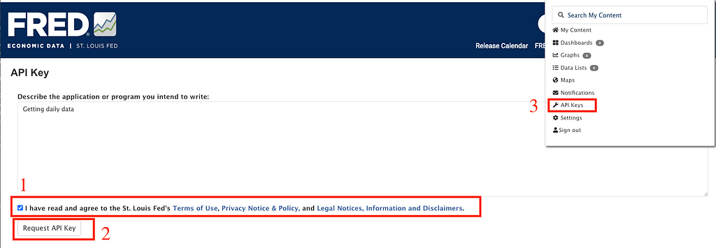
5. Copy your API Key
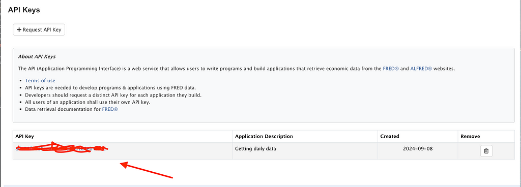
Then, you’ll see your API key displayed. You’ll need to copy it into the Python script to make requests to the FRED St. Louis API (next section).
Fetching the data
Now that we have our API key, we can retrieve data from the FRED API. The first step is to store your API key in a .env file. In your terminal, run touch .env to create the file. Then, open the .env file and add your API key like this:
API_KEY=your_api_key_here
You are now ready to retrieve data from the FRED API.
import requests
import pandas as pd
from dotenv import load_dotenv
import os
load_dotenv()
API_KEY = os.getenv("API_KEY")
FRED_LIST= 'fred_daily_series_list.csv'

def get_daily_series(api_key):
    base_url = "https://api.stlouisfed.org/fred/tags/series"
    params = {
        "api_key": api_key,
        "tag_names": "daily",
        "file_type": "json",
        "limit": 1000,
        "offset": 0
    }

    all_series = []

    while True:
        try:
            response = requests.get(base_url, params=params)
            response.raise_for_status()
            data = response.json()

            if "seriess" in data:
                series_chunk = data["seriess"]
                all_series.extend(series_chunk)

                if len(series_chunk) < params["limit"]:
                    break
                params["offset"] += params["limit"]
            else:
                break
        except requests.exceptions.RequestException as e:
            print(f"Error fetching data: {e}")
            break
    return all_series


daily_series = get_daily_series(API_KEY)
df = pd.DataFrame(daily_series)
print(f"\nNumber of FRED series with daily data: {len(df)}\n")
df = df[['id']]
df.to_csv(FRED_LIST, index=False)
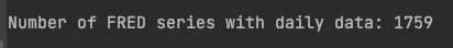
There are 1759 different series with daily data, which is significant. We have plenty to train a complex model.
Then, we’ll fetch the actual series one by one from 2014-10-01 to 2024-09-05 for approximately 10 years of data. You can adjust the date range according to your preferences by changing START_DATE and END_DATE. Each series will be saved as a CSV file in the folder data.
import os
from io import StringIO

START_DATE = '2014-10-01'
END_DATE = '2024-09-05'
DATA_FOLDER = 'data'

def fetch_data(series_id):
    request = f"https://fred.stlouisfed.org/graph/fredgraph.csv?id={series_id}"
    request += f"&cosd={START_DATE}"
    request += f"&coed={END_DATE}"
    try:
        response = requests.get(request)
        response.raise_for_status()
        df = pd.read_csv(StringIO(response.text), parse_dates=True)
        df.rename(
            columns={
                df.columns[0]: 'ds',
                df.columns[1]: 'value',
            },
            inplace=True,
        )
        return series_id, df
    except requests.RequestException as e:
        print(f"Error fetching data for {series_id}: {e}")
        return series_id, None

df = pd.read_csv(FRED_LIST)
os.makedirs(DATA_FOLDER, exist_ok=True)
series_ids = df['id'].tolist()

for series_id in series_ids:
    series_id, data = fetch_data(series_id)
    if data is not None:
        filename = os.path.join(DATA_FOLDER, f"{series_id}.csv")
        data.to_csv(filename, index=False)
As mentioned at the beginning of the article, we will train a model using the NeuralForecast library with data from FRED. To meet NeuralForecast’s input requirements, we need to prepare our data in a specific format.
Y_df is a dataframe with three columns: unique_id with a unique identifier for each time series, a column ds with the datestamp and a column y with the values of the series.
This is why we renamed the first column to ds (df.columns[0] = 'ds'). The FRED API returns dates in the first column, and NeuralForecast requires this specific column name for datestamps as mentioned above.
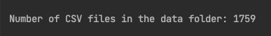
Next, we’ll count the number of CSV files in our data folder to verify that the API successfully fetched all 1759 data series we previously identified.
def count_csv_files(folder_path):
    csv_count = 0
    for filename in os.listdir(folder_path):
        if filename.endswith('.csv'):
            csv_count += 1
    return csv_count

num_csv_files = count_csv_files(DATA_FOLDER)
print(f"\nNumber of CSV files in the {DATA_FOLDER} folder: {num_csv_files}\n")
We do a quick exploratory data analysis with one data series.
file_path = os.path.join(DATA_FOLDER, 'AAA10Y.csv')
df = pd.read_csv(file_path)

print("\nLast 10 rows of AAA10Y:")
print("=" * 30)
print(df.tail(10))
print("=" * 30)
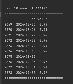
We have a missing value for Labor Day, which is acceptable since the stock market is closed on this holiday. With that in mind, we’ll prepare and clean the data in the following steps. This process is crucial to ensure accurate and robust results from our machine learning models.
Preparing the data
1. Determining NYSE trading days
We define a function that returns the dates when the New York Stock Exchange (NYSE) is open.
import pandas_market_calendars as mcal
from typing import Optional

def obtain_market_dates(start_date: str, end_date: str, market : Optional[str] = "NYSE") -> pd.DataFrame:
    nyse = mcal.get_calendar(market)
    market_open_dates = nyse.schedule(
        start_date=start_date,
        end_date=end_date,
    )
    return market_open_dates

market_dates = obtain_market_dates(START_DATE,END_DATE)
2- Removing missing values
We mask (temporarily) the empty cells, None values, or entries containing only a . in our dataset. We will replace them in the next step.
def replace_empty_data(df : pd.DataFrame) -> pd.DataFrame:
    mask = df.isin(["", ".", None])
    rows_to_remove = mask.any(axis=1)
    return df.loc[~rows_to_remove]

df_cleaned = replace_empty_data(df_correct_dates)
3- Replacing missing values
We replace any missing values with the previous value in the series, or assign 0 if it’s the first value. For robustness, we set a MAX_MISSING_DATA threshold of 2%, though this could be increased to 5% without significant issues. Any series with more than 2% missing data is discarded and not used in our model.
from typing import Union, Tuple
import logging
MAX_MISSING_DATA = 0.02

def handle_missing_data(
        data: pd.DataFrame,
        market_open_dates : pd.DataFrame,
        data_series : str
) -> Tuple[Union[None,pd.DataFrame], Union[pd.DataFrame, None]]:
    modified_data = data.copy()
    market_open_dates["count"] = 0
    date_counts = data['ds'].value_counts()

    market_open_dates["count"] = market_open_dates.index.map(
        date_counts
    ).fillna(0)

    missing_dates = market_open_dates.loc[
        market_open_dates["count"] < 1
    ]

    if not missing_dates.empty:
        max_count = (
            len(market_open_dates)
            * MAX_MISSING_DATA
        )

        if len(missing_dates) > max_count:
            logging.warning(
                f"For the series {data_series} there are "
                f"{len(missing_dates)} data points missing, which is greater than the maximum threshold of "
                f"{MAX_MISSING_DATA * 100}%"
            )
            return pd.DataFrame(), None
        else:
            for date, row in missing_dates.iterrows():
                modified_data = insert_missing_date(
                    modified_data, date, 'ds'
                )
    return modified_data, missing_dates


def insert_missing_date(
        data: pd.DataFrame,
        date: str,
        date_column: str
) -> pd.DataFrame:
    date = pd.to_datetime(date)
    if date not in data[date_column].values:
        prev_date = (
            data[data[date_column] < date].iloc[-1]
            if not data[data[date_column] < date].empty
            else data.iloc[0]
        )
        new_row = prev_date.copy()
        new_row[date_column] = date
        data = (
            pd.concat([data, new_row.to_frame().T], ignore_index=True)
            .sort_values(by=date_column)
            .reset_index(drop=True)
        )
    return data
4- Processing individual data series
We apply all our previous steps to each data series individually. When we encounter the S&P 500 series (detected via if 'SP500.csv in csv_file:), we save it directly in our model_data variable, as this will be the target output for our forecasting model.
import glob
processed_dataframes = []
market_dates_only = market_dates.index.date

for csv_file in glob.glob(os.path.join(DATA_FOLDER, "*.csv")):

    df = pd.read_csv(csv_file)
    df['ds'] = pd.to_datetime(df['ds'])
    df_correct_dates = df[df['ds'].dt.date.isin(market_dates_only)]
    df_cleaned = replace_empty_data(df_correct_dates)
    processed_df, missing_dates = handle_missing_data(df_cleaned,market_dates,os.path.basename(csv_file).split('.')[0])
    if not processed_df.empty:
        processed_df['ds'] = pd.to_datetime(processed_df['ds'])
        if not missing_dates.empty:
            for missing_date in missing_dates.index:
                missing_date = pd.to_datetime(missing_date)
                if missing_date in processed_df['ds'].values:
                    continue

                previous_day_data = processed_df[processed_df['ds'] < missing_date].tail(1)

                if previous_day_data.empty:
                    new_row = pd.DataFrame({'ds': [missing_date], 'value': [0]})
                else:
                    new_row = previous_day_data.copy()
                    new_row['ds'] = missing_date

                processed_df = pd.concat([processed_df, new_row]).sort_values('ds').reset_index(drop=True)
        if 'SP500.csv' in csv_file:
            model_data = processed_df.rename(columns={'value': 'price'}).reset_index(drop=True)
        processed_dataframes.append(processed_df.reset_index(drop=True))

print(f"\nNumber of data series remaining after cleanup: {len(processed_dataframes)}\n")
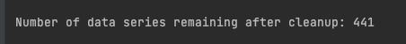
We retained 441 out of 1759 series after removing those with excessive missing values. This reduction could partly be explained by our 10-year date range. However, the remaining 441 series still form a robust dataset for our deep learning model.
5- Dimensionality reduction
Ideally, we should make our data stationary before performing dimensionality reduction, as detailed in this article. However, we’ll skip this step for simplicity.
Keep in mind that dimensionality reduction is beneficial but optional. While we could train our model using all individual data series, many are likely highly correlated (e.g., stock indices like Dow, S&P 500, and Russell). By reducing dimensions, we can enhance both the robustness and performance of our model.
from sklearn.preprocessing import StandardScaler
from sklearn.decomposition import PCA
EXPLAINED_VARIANCE = .9
MIN_VARIANCE = 1e-10

combined_df = pd.concat([df.set_index('ds') for df in processed_dataframes], axis=1)
combined_df.columns = [f'value_{i}' for i in range(len(processed_dataframes))]

X = combined_df.values
scaler = StandardScaler()
X_scaled = scaler.fit_transform(X)


pca = PCA(n_components=EXPLAINED_VARIANCE, svd_solver='full')
X_pca = pca.fit_transform(X_scaled)

X_pca = X_pca[:, pca.explained_variance_ > MIN_VARIANCE]


pca_df = pd.DataFrame(
    X_pca,
    columns=[f'PC{i+1}' for i in range(X_pca.shape[1])]
)

print(f"\nOriginal number of features: {combined_df.shape[1]}")
print(f"Number of components after PCA: {pca_df.shape[1]}\n")

model_data = model_data.join(pca_df)
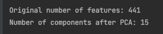
We used principal components analysis (PCA) for dimensionality reduction and used an EXPLAINED_VARIANCE of 90%. This means that the algorithm will retain enough principal components to explain 90% of the variance in the original features.
It’s worth noting that while we used PCA for dimensionality reduction, which is an effective, widely-used technique and good enough for our use-case, it primarily considers linear relationships between features. However, we will use a transformer-based model in the next step which is designed to capture non-linear relationships in the data. Consequently, PCA may oversimplify or omit complex, non-linear patterns that the model is designed to detect.
Training the model
We will forecast the S&P 500 index using our data obtained from FRED. For this purpose, we’ll employ the Temporal Fusion Transformer model (TFT) available in the NeuralForecast library. It’s worth noting that any forecasting model from NeuralForecast that incorporates historical exogenous variables would be suitable for this task.
This example demonstrates a basic forecasting model. For a more comprehensive and detailed approach, please refer to this article on the subject.
from neuralforecast.models import TFT
from neuralforecast import NeuralForecast

TRAIN_SIZE = .90
model_data['unique_id'] = 'SPY'
model_data['price'] = model_data['price'].astype(float)
model_data['y'] = model_data['price'].pct_change()
model_data = model_data.iloc[1:]
hist_exog_list = [col for col in model_data.columns if col.startswith('PC')]

train_size = int(len(model_data) * TRAIN_SIZE)
train_data = model_data[:train_size]
test_data = model_data[train_size:]

model = TFT(
    h=1,
    input_size=24,
    hist_exog_list=hist_exog_list,
    scaler_type='robust',
    max_steps=20
)

nf = NeuralForecast(
    models=[model],
    freq='D'
)

nf.fit(df=model_data)
Code explanation :
- We train our model using the daily return from the S&P 500 index: model_data['y] = model['price'].pct_change()
- We set a 1-day ahead forecasting horizon: h=1
- Following NeuralForecast data requirements,y represents our forecast target (S&P 500 daily return)
- According to NeuralForecast guidelines, we specify historical variables using the hist_exog_list parameter. For our model, this list contains the principal components we calculated earlier.
Next, we generate one-day-ahead predictions for each data point in the test set, forecasting the S&P 500 daily returns. We then convert these return forecasts back to price forecasts by multiplying each predicted return by the previous day’s price.
y_hat_test_ret = pd.DataFrame()
current_train_data = train_data.copy()

y_hat_ret = nf.predict(current_train_data)
y_hat_test_ret = pd.concat([y_hat_test_ret, y_hat_ret.iloc[[-1]]])

for i in range(len(test_data) - 1):
    combined_data = pd.concat([current_train_data, test_data.iloc[[i]]])
    y_hat_ret = nf.predict(combined_data)
    y_hat_test_ret = pd.concat([y_hat_test_ret, y_hat_ret.iloc[[-1]]])
    current_train_data = combined_data

predicted_returns = y_hat_test_ret['TFT'].values

predicted_prices_ret = []
for i, ret in enumerate(predicted_returns):
    if i == 0:
        last_true_price = train_data['price'].iloc[-1]
    else:
        last_true_price = test_data['price'].iloc[i-1]
    predicted_prices_ret.append(last_true_price * (1 + ret))
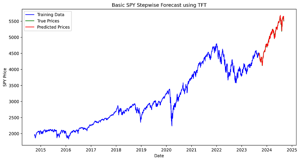
To visualize our results, we create a graph comparing the model’s predictions (red) with the actual S&P 500 prices (green).
import matplotlib.pyplot as plt
true_values = test_data['price']

plt.figure(figsize=(12, 6))
plt.plot(train_data['ds'], train_data['price'], label='Training Data', color='blue')
plt.plot(test_data['ds'], true_values, label='True Prices', color='green')
plt.plot(test_data['ds'], predicted_prices_ret, label='Predicted Prices', color='red')
plt.legend()
plt.title('Basic SPY Stepwise Forecast using TFT')
plt.xlabel('Date')
plt.ylabel('SPY Price')
plt.savefig('spy_forecast_chart.png', dpi=300, bbox_inches='tight')
plt.close()
Conclusion
This is it! We’ve successfully learned how to acquire and use free, reliable financial and economic data for our stock forecasting model. Specifically, we covered:
- Retrieving high-quality financial and economic data from the FRED API at no cost
- Processing and cleaning the data for machine learning use
- Implementing dimensionality reduction using PCA
- Training a stock forecasting model with our acquired data
In upcoming articles, we’ll expand our approach by:
- Incorporating additional data sources, such as social media sentiment analysis
- Exploring more sophisticated dimensionality reduction techniques tailored for deep learning models
Stay tuned for more insights!
Ready to put these concepts into action? You can find the complete code implementation here.
Liked this article? Show your support!
👏 Clap it up to 50 times
🤝 Send me a LinkedIn connection request to stay in touch
Your support means everything! 🙏
Get Free, and Reliable Financial Market Data — Machine Learning-Ready was originally published in Level Up Coding on Medium, where people are continuing the conversation by highlighting and responding to this story.
This content originally appeared on Level Up Coding - Medium and was authored by Philippe Ostiguy, M. Sc.
Philippe Ostiguy, M. Sc. | Sciencx (2024-09-16T02:21:51+00:00) Get Free, and Reliable Financial Market Data — Machine Learning-Ready. Retrieved from https://www.scien.cx/2024/09/16/get-free-and-reliable-financial-market-data-machine-learning-ready/
Please log in to upload a file.
There are no updates yet.
Click the Upload button above to add an update.