This content originally appeared on Level Up Coding - Medium and was authored by Pranjal Saxena
Building Algorithmic Trading Models with LSTMs

Algorithmic trading, also called “algo trading,” is the use of computer programs to execute trading strategies automatically. These strategies are built on predefined rules and use vast amounts of market data.
With the rise of technology, algorithmic trading has become a game-changer in financial markets. It helps traders take advantage of opportunities in real time. By using algorithms, traders can avoid emotional biases and stick to their strategies, which often leads to more consistent returns.
Deep learning is a type of machine learning that has transformed many industries, including finance. In the world of trading, deep learning helps identify hidden patterns in stock prices. These models are great at handling complex relationships and analyzing time-series data, which makes them ideal for stock price prediction.
By using deep learning, we can teach a model to predict future prices based on past data. This prediction helps us make more informed trading decisions. Unlike traditional models, deep learning can learn from intricate data patterns, which gives it a significant edge when trading in volatile markets.
To train a deep learning model, we need accurate and reliable data. This is where EODHD comes in. The EODHD API provides us with easy access to financial market data, including historical stock prices.
With EODHD, we can fetch historical data of any stock we’re interested in. It’s fast, easy to use, and reliable. This makes it a perfect choice for our deep learning project. Whether you’re building a small experiment or a large-scale trading system, EODHD has you covered.
In this article, we’ll cover the basics of deep learning for algorithmic trading. We’ll start by understanding how neural networks work. Then, we’ll dive into their components like the input layer, hidden layers, activation functions, and loss functions. Once we’ve covered the theory, we’ll put it all into practice with Python. You’ll learn how to fetch data using EODHD and build a stock price prediction model with both Keras and PyTorch.
By the end, you’ll have a hands-on example of how deep learning can enhance your trading strategies.
Neural Networks: Basics and Working
Imagine trying to predict stock prices based on hundreds of factors — past prices, market news, interest rates, global events. For humans, it’s a daunting task. Neural networks are like super-smart assistants that help us make sense of this data chaos. Inspired by the human brain, they learn by connecting different bits of information, just like how our brain connects neurons to form thoughts.
At its core, a neural network is a collection of “neurons” grouped into layers. They’re not biological, but think of them as tiny, digital decision-makers. Each one takes in some data, processes it, and then sends a signal to the next layer, just like neurons passing signals in your brain. With enough layers working together, these networks can learn very complex relationships — just the thing we need to figure out the financial markets!
Neural Network Components
1. Input Layer, Hidden Layers, and Output Layer
Neural networks are organized into layers. There’s the input layer, which takes in all the raw data — think of it as the “senses” of the network. It sees the past stock prices, the latest news sentiment, or anything else we want it to look at.
Next come the hidden layers. These are where the magic happens. In these layers, the neurons get to work crunching numbers and making sense of the data. They identify relationships — like when a price usually goes up after certain market conditions. We can have one or many hidden layers, depending on how complex we want our network to be.
Finally, we have the output layer, which tells us the result — maybe the predicted price of a stock or whether we should buy or sell. Think of the output layer as the final decision-maker, based on everything the network has learned.
2. Working of a Neural Network
Neural networks are all about learning. Here’s how it works:
- Forward Propagation: Imagine we have a neural network trying to predict if a stock will rise. It starts by taking the input — historical data, current market stats, etc. This data passes through the hidden layers, where each neuron processes it and decides how important each factor is. Finally, it reaches the output layer, where it gives us a prediction, like “the price will go up by 2% tomorrow.”
- Weights and Biases: Weights are like the importance level each neuron assigns to the incoming data. For example, if historical stock prices are very important for prediction, the network gives those more “weight.” Biases are little adjustments added to fine-tune the results. Together, weights and biases help the network figure out what matters the most.
3. Activation Functions
But here’s where things get interesting — neurons need to decide when to activate or “fire.” This is done using something called activation functions. Think of activation functions as decision-makers.
- If the neuron sees something important, it “fires” — much like if you heard great news that makes you excited.
- Common activation functions include ReLU (Rectified Linear Unit), which “fires” if something is positively contributing, and Sigmoid, which can squish outputs into values between 0 and 1.
Without activation functions, the neural network would be just a fancy calculator. These functions help the network make smart decisions about which data matters the most.
4. Forward Propagation
When the network first makes predictions, it’s called forward propagation. It’s like taking your first guess about which way the stock market will move — based on what you’ve learned so far.
5. Backpropagation
Of course, the first guess isn’t always correct — just like a first prediction about the market might be way off. This is where backpropagation comes in. It’s like the neural network’s way of learning from its mistakes. It calculates how far off the prediction was and then adjusts the weights and biases to improve the next time.
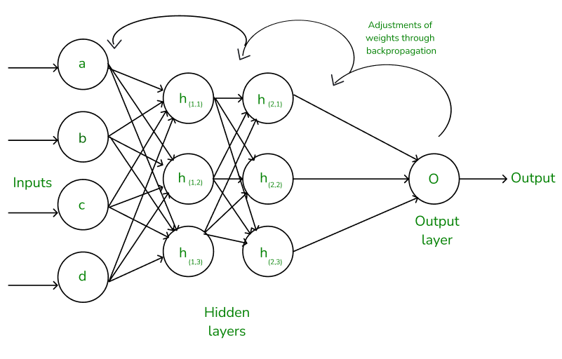
Think of backpropagation as a feedback loop — like if you bought a stock and it went down, you learn from it. The network does this, but thousands of times faster, getting better and better at predicting prices.
6. Loss Functions
Imagine your neural network predicting the next day’s stock price. Sometimes, it gets close; other times, it’s way off. The loss function is what we use to measure how far off the mark the prediction is. It’s like a scorekeeper, telling us how well — or poorly — the model is doing. The smaller the “loss,” the better our network is predicting.
In simpler terms, a loss function is just a way to measure the error of a prediction. If the network predicts that a stock will increase by $10 but it actually only increases by $5, the loss function tells the network, “Whoa, you overshot it by $5!” The goal is to minimize this error, so the network gets better at predicting over time.
Different tasks need different types of loss functions. Since we’re predicting stock prices, we’re dealing with regression, where our output is a number. The most commonly used loss function for regression is:
- Mean Squared Error (MSE): MSE is like saying, “Let’s find out how much we’re off on average, square the errors (to make sure they’re positive), and then take the mean.” It’s simple but powerful. The lower the MSE, the closer our predictions are to the actual values.
- For classification tasks — like predicting if the market will go up or down — we’d use a different type of loss function called Cross-Entropy Loss. But for now, since we’re focused on predicting prices, MSE is our go-to.
7. Optimizers and Gradient Descent
If a loss function is the scorekeeper, the optimizer is the coach. It tells the network how to adjust its game plan to reduce errors. Optimizers adjust the weights and biases of the neural network to minimize the loss.
The most popular optimization technique in neural networks is Gradient Descent. Here’s how it works:
Picture yourself at the top of a hill, trying to get to the lowest point — the “valley.” The valley represents the minimum loss (or error). Gradient descent helps the neural network move step by step downhill to reach that lowest point. The direction and size of each step are calculated based on the slope — just like how you’d carefully take small steps on a steep slope to avoid falling.
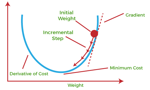
The idea is simple: measure the loss (how high we are on the hill), find out which way leads downhill, and then take a step in that direction. Repeat this over and over until we reach the lowest point, where the network makes the best possible predictions.
Gradient descent has evolved over time, and now we have several versions of it:
- Stochastic Gradient Descent (SGD): It takes small steps, adjusting weights after each individual prediction. This helps to avoid getting stuck in a local minimum.
- Adam Optimizer: Adam stands for Adaptive Moment Estimation. It’s like a smarter version of gradient descent, adjusting the learning rate on the go. It’s faster and often more efficient for deep learning, making it a favorite choice among traders and developers.
Building a Stock Price Prediction Model Using Python
1. Fetching Stock Data Using EODHD API
To build our predictive model, we need historical stock data. EODHD makes it easy to access end-of-day (EOD) data and other financial metrics via an API. Let’s walk through the process of fetching this data so we can feed it into our deep learning model.
First, we need an API key from EODHD. You can register on their platform and get an API key to access the data. Once you have your API key, you can use it to pull stock data using Python. Here’s a simple script to get you started.
import requests
import pandas as pd

API_KEY = 'YOUR_API_KEY'
SYMBOL = 'NVDA'  # Ticker symbol for Nvidia Stock.
URL = f'https://eodhistoricaldata.com/api/eod/{SYMBOL}?api_token={API_KEY}&fmt=json'

# Make the request
response = requests.get(URL)

# Check if the request was successful
if response.status_code == 200:
    data = response.json()
    # Load data into a DataFrame
    df = pd.DataFrame(data)
    # Convert the date column to datetime
    df['date'] = pd.to_datetime(df['date'])
    print(df.tail())
else:
    print("Failed to fetch data. Status code:", response.status_code)

2. Preparing Data for Deep Learning
Once we have our historical data, we need to prepare it for our deep learning model. Preparing data for deep learning involves a few simple but critical steps: cleaning, normalizing, and creating sequences.
Data Cleaning
- Start by checking for missing values. Missing values can interfere with the model’s ability to learn effectively.
- Drop rows with missing data or fill them with a suitable replacement like the mean or median value.
# Check for missing values and handle them
df = df.dropna()
Normalizing the Data
Neural networks work best when the data is scaled. Since we’re dealing with stock prices, the values can be quite large. To make it easier for the network to understand the data, we normalize it to a smaller range, usually between 0 and 1.
from sklearn.preprocessing import MinMaxScaler

scaler = MinMaxScaler(feature_range=(0, 1))
scaled_data = scaler.fit_transform(df[['adjusted_close']])
Here, we use MinMaxScaler from scikit-learn to scale the data between 0 and 1.
3. Creating Input Sequences
Since we’re dealing with time-series data, we need to create sequences that help the network learn patterns over time. For example, we can use the past 30 days to predict the next day’s stock price.
import numpy as np

sequence_length = 30
X = []
y = []

for i in range(sequence_length, len(scaled_data)):
    X.append(scaled_data[i-sequence_length:i, 0])
    y.append(scaled_data[i, 0])

# Convert lists to numpy arrays
X, y = np.array(X), np.array(y)

# Reshape X to be suitable for LSTM (samples, time steps, features)
X = np.reshape(X, (X.shape[0], X.shape[1], 1))
In this code:
- X represents the sequences of stock prices over 30 days.
- y represents the next day’s price.
- We reshape X to match the input shape expected by LSTM models, which usually requires [samples, time steps, features] format.
Why Sequence Data?
Stock prices over time are highly correlated — today’s price is influenced by yesterday’s, and so on. By using sequences, we allow our model to learn these time-based dependencies.
Implementing the Deep Learning Model: Keras and PyTorch
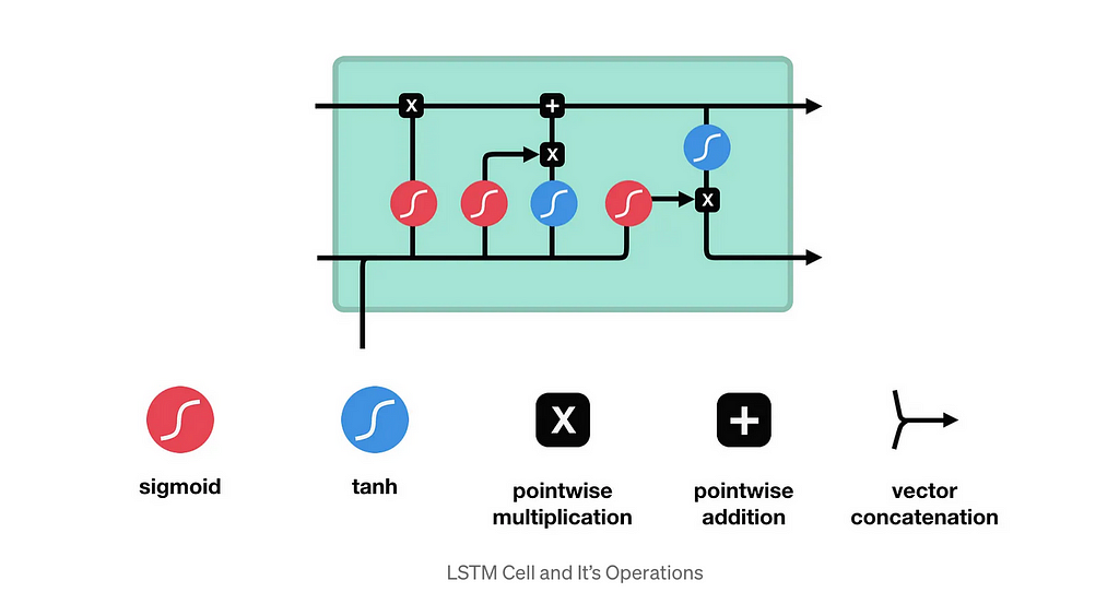
In this section, we’ll build two deep learning models for stock price prediction: one using Keras and the other with PyTorch. We’ll focus on using LSTMs (Long Short-Term Memory) networks, which are particularly effective for time-series data like stock prices.
Let’s start by implementing our LSTM model using Keras and then replicate a similar approach using PyTorch.
1. Building an LSTM Model with Keras
Keras is a high-level deep learning library that makes building neural networks straightforward and user-friendly. Here, we’ll create an LSTM model to predict stock prices based on our historical data.
from keras.models import Sequential
from keras.layers import LSTM, Dense, Dropout

# Initialize the LSTM model
model = Sequential()

# Add the LSTM layer with 50 units, input shape matches our sequences (30 timesteps, 1 feature)
model.add(LSTM(units=50, return_sequences=True, input_shape=(X.shape[1], 1)))
model.add(Dropout(0.2))  # Dropout layer to prevent overfitting

# Add another LSTM layer
model.add(LSTM(units=50, return_sequences=False))
model.add(Dropout(0.2))

# Add a Dense output layer with one unit to predict the closing price
model.add(Dense(units=1))

# Compile the model using Adam optimizer and Mean Squared Error loss function
model.compile(optimizer='adam', loss='mean_squared_error')

# Train the model and store the training history
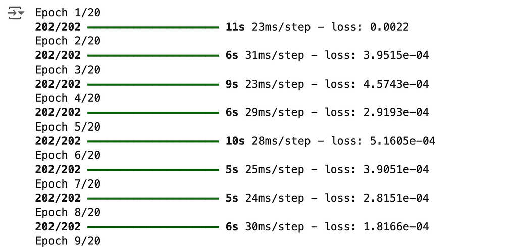
history = model.fit(X, y, epochs=20, batch_size=32)

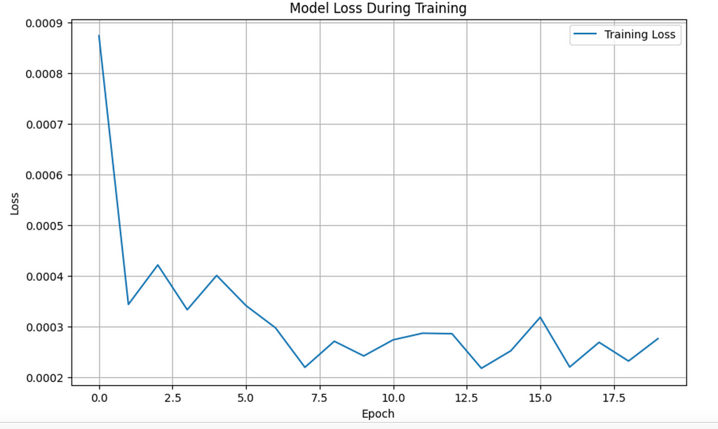
# Plotting the loss curve
plt.figure(figsize=(10, 6))
plt.plot(history.history['loss'], label='Training Loss')
plt.title('Model Loss During Training')
plt.xlabel('Epoch')
plt.ylabel('Loss')
plt.legend()
plt.grid(True)
plt.show()
Explanation
- LSTM Layers: We added two LSTM layers, each with 50 units (neurons). LSTMs are great for time-series data because they remember important sequences over time.
- Dropout Layers: To avoid overfitting — where our model performs well on training data but poorly on new data — we use Dropout. This randomly drops some neurons during training to make the model more robust.
- Dense Layer: The output layer uses Dense(units=1), meaning it predicts one value: the next day’s stock price.
- Optimizer and Loss Function: We use Adam as the optimizer because it’s adaptive and efficient for deep learning. The Mean Squared Error (MSE) is our loss function since we’re predicting continuous values.
2. Building a Model Using PyTorch
Now let’s create a similar model using PyTorch. PyTorch is a more flexible deep learning library compared to Keras and is often used for more custom models.
import torch
import torch.nn as nn
import torch.optim as optim
from torch.utils.data import DataLoader, TensorDataset

# Convert numpy arrays to torch tensors
X_train = torch.from_numpy(X).float()
y_train = torch.from_numpy(y).float()

# Define LSTM model using PyTorch
class LSTMModel(nn.Module):
    def __init__(self, input_size=1, hidden_size=50, num_layers=2):
        super(LSTMModel, self).__init__()
        self.lstm = nn.LSTM(input_size, hidden_size, num_layers, batch_first=True)
        self.fc = nn.Linear(hidden_size, 1)

    def forward(self, x):
        lstm_out, _ = self.lstm(x)
        output = self.fc(lstm_out[:, -1, :])  # Get the output from the last time step
        return output

# Instantiate the model, define loss and optimizer
model = LSTMModel()
criterion = nn.MSELoss()
optimizer = optim.Adam(model.parameters(), lr=0.001)

# Create DataLoader to handle batches
dataset = TensorDataset(X_train, y_train)
loader = DataLoader(dataset, batch_size=32, shuffle=True)

# Train the model
epochs = 20
for epoch in range(epochs):
    for batch in loader:
        X_batch, y_batch = batch
        optimizer.zero_grad()
        y_pred = model(X_batch)
        loss = criterion(y_pred, y_batch)
        loss.backward()
        optimizer.step()

    print(f"Epoch {epoch+1}/{epochs}, Loss: {loss.item()}")
Explanation
- LSTM Model: We define our LSTM model as a class, which includes an LSTM layer and a fully connected layer to generate predictions.
- LSTM Layer: Like in Keras, we use 50 units in the LSTM layer, with 2 layers in total.
- Fully Connected Layer: After the LSTM, we use a fully connected layer to reduce the output to a single prediction value.
- Optimizer and Loss Function: We use Adam for optimization and MSELoss for measuring the error.
Training Loop
We convert our data into DataLoader batches to train the model more efficiently. During each epoch, we pass each batch through the model, compute the loss, and adjust the weights using backpropagation.
3. Evaluation of Models
Once both models are trained, we evaluate them to see how well they predict new data. We can use metrics like Root Mean Squared Error (RMSE) to quantify the model’s performance.
Evaluating the Keras Model
# Use the model to predict and then compute RMSE
predicted_prices = model.predict(X)
predicted_prices = scaler.inverse_transform(predicted_prices)
rmse = np.sqrt(np.mean((predicted_prices - y_actual) ** 2))
print("RMSE for Keras Model:", rmse)
Evaluating the PyTorch Model
with torch.no_grad():
    y_pred = model(X_train)
    y_pred = y_pred.numpy()
    y_pred = scaler.inverse_transform(y_pred)
    rmse = np.sqrt(np.mean((y_pred - y_actual) ** 2))
    print("RMSE for PyTorch Model:", rmse)
Why LSTM?
We use LSTMs because they can remember important trends over a longer period of time. This makes them highly effective for financial time-series data like stock prices, which often have long-term dependencies.
Why Keras and PyTorch?
- Keras is great for quickly building models with fewer lines of code. It’s simple and straightforward.
- PyTorch gives you more control and flexibility, which is beneficial for more advanced projects or custom layers.
Conclusion
In this article, we demonstrated how to use deep learning for algorithmic trading. We explored neural networks, activation functions, loss functions, and optimization.
Using EODHD data, we built LSTM models with Keras and PyTorch to predict stock prices. Deep learning helps identify complex market patterns, making it a valuable tool for traders.
With this knowledge, you’re ready to explore deeper possibilities in financial predictions and make more informed trading decisions.
Algorithmic Trading with Deep Learning: Utilizing Historical Stock Price Data via API was originally published in Level Up Coding on Medium, where people are continuing the conversation by highlighting and responding to this story.
This content originally appeared on Level Up Coding - Medium and was authored by Pranjal Saxena
Pranjal Saxena | Sciencx (2024-10-08T16:38:46+00:00) Algorithmic Trading with Deep Learning: Utilizing Historical Stock Price Data via API. Retrieved from https://www.scien.cx/2024/10/08/algorithmic-trading-with-deep-learning-utilizing-historical-stock-price-data-via-api/
Please log in to upload a file.
There are no updates yet.
Click the Upload button above to add an update.
