This content originally appeared on HackerNoon and was authored by Economic Hedging Technology
Table of Links
1.2 Asymptotic Notation (Big O)
1.5 Monte Carlo Simulation and Variance Reduction Techniques
- Literature Review
- Methodology
3.2 Theorems and Model Discussion
3.2 THEOREMS AND MODEL DISCUSSION
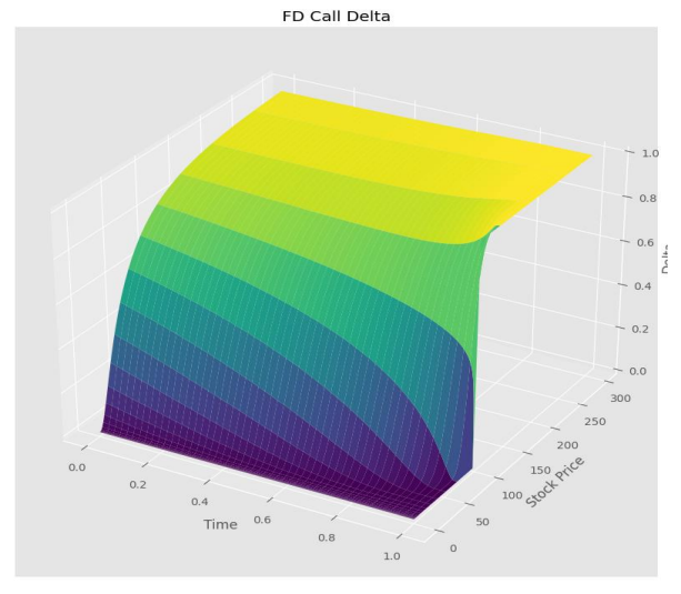
The three steps we take are outlined in Theorems 1 through 3. We begin by deriving an equation for the hedge error variance in the case when each call position in the portfolio has a standard delta hedge applied to it [22]. Following that, To protect against changes in the value of the option portfolio, we create an analogous formula for the scenario in which an arbitrary portfolio in the underlying values is retained [23]. As a result, we are able to show how selecting the right hedge portfolio helps lower hedge error variances. We last provide our major theoretical finding, which demonstrates that by focusing only on the linear and higher order exposures to the systematic risk factor [24], it becomes possible to design a perfect static hedge portfolio in finite time, provided that the portfolio size grows infinitely [25].
\
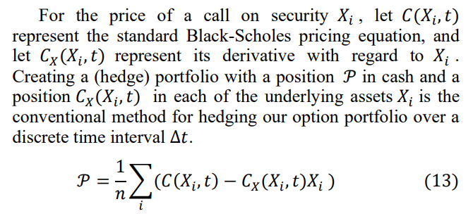
\ Hedge error is defined by ∆𝐻 as
\

\ The hedge portfolio is the total of the hedge portfolios for each individual position when using the hedging approach described above [26]. We create a power series by expanding the hedge mistake (14) [27]. Regarding the duration of the hedging period ∆𝑡, See Leland (1985) as well as Mello and Neuhaus (1998). The predicted hedging error and its variation under the current conventional delta hedging method are as follows [28].
\ Theorem 1: The hedging error ∆𝐻 in (14), which is obtained through delta hedging of the individual option holdings, satisfies
\
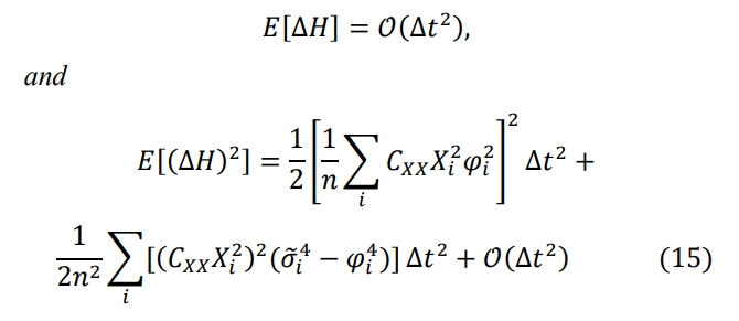
\ Essentially, for N = 1, we obtain the square of the option's gamma, which is the well-known calculation for the hedge error variance [3].
\
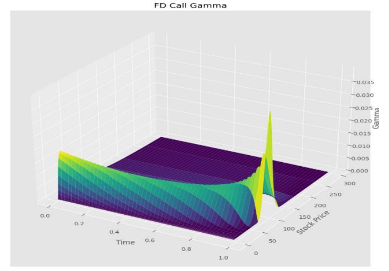
\ This variance's explicit representation clearly indicates that the option portfolio's return is no longer reproduced riskfree in a defined amount of time using the Black-Scholes hedging strategy. Thus, it appears that the option portfolio does not have a unique preference free pricing.
\
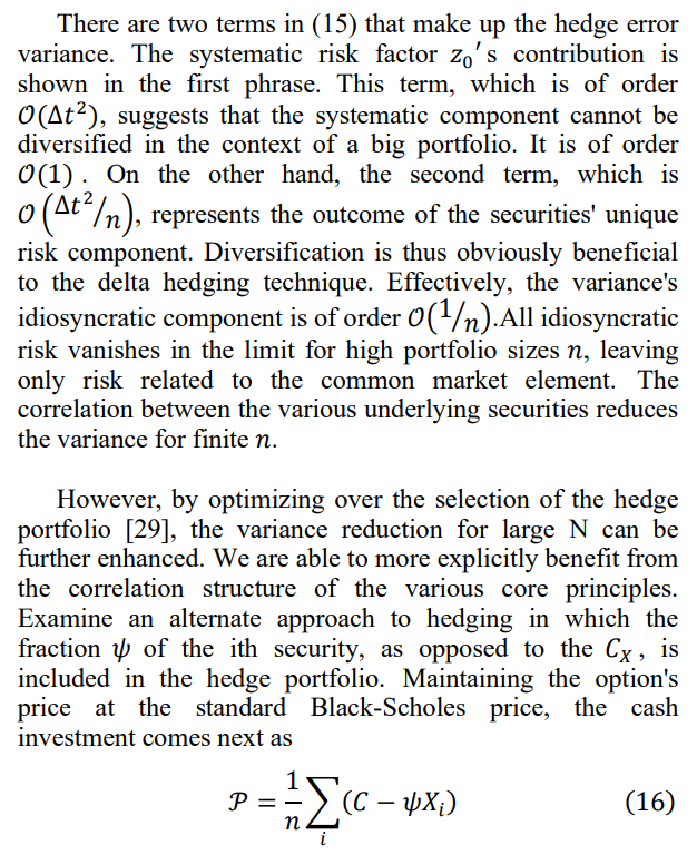
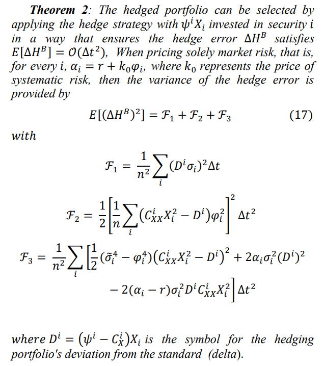
\ With this unconventional approach to hedging, we get the following outcome for the hedge error variance.
\
\
\
\
\
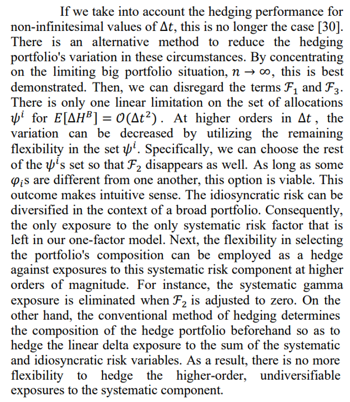
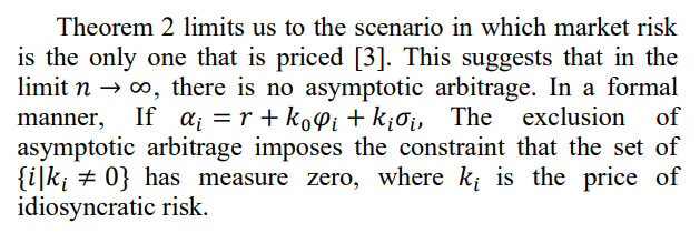
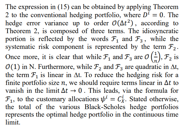
\ There is a trade-off between insuring all idiosyncratic risk (in the limit 𝑛∆𝑡 → 0 , the traditional Black-Scholes technique) and hedging market risk exclusively (in the limit 𝑛∆𝑡 →∞) for finite portfolio size 𝑛 and finite revision time ∆𝑡. Clearly, with bigger portfolio sizes and revision intervals, there are more departures from the traditional hedging technique in terms of hedge ratios and variance reduction. Now that we have established the general conclusion, we may argue that it is better to hedge higher order systematic risk rather than linear idiosyncratic risk in big option portfolios. The subsequent theorem does this.
\
\ One can demonstrate a similar outcome if idiosyncratic risk is valued [3]. In that scenario, the quantity of securities required to build the hedging portfolio grows quadratically with 𝑎. Furthermore, there are now prospects for arbitrage since the projected return of this hedging approach need not be zero. This is to be expected because arbitrage is possible in a market structure that doesn't even have options [24].
\
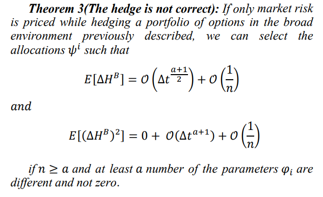
\ Theorem 3's result shows that if the 𝜑𝑖 s are different, we can create a riskless hedging strategy for finite time ∆𝑡 in the limit 𝑛 →∞. Stated otherwise, the risk incurred by switching to a discrete time setup entirely disappears: by selecting the suitable non-standard hedging approach, the systematic risk component can be eliminated to any arbitrary order of ∆𝑡. Diversification causes the idiosyncratic risk component to vanish at the same time. The hedge portfolio is selected so that, up to a high enough order in ∆t, its expectation conditional on the systematic risk component corresponds with its unconditional expectation. This is the key to the demonstration. By matching the higher order properties of the systematic risk exposure, this may be proven. The portfolio loadings 𝜓 𝑖 must be subject to a series of restrictions in order to meet the two sorts of expectations. In the 𝜓 𝑖 s, each of these restrictions is linear. The coefficients of these constraints entail powers of the systematic volatility 𝜑𝑖 and higher order derivatives of the Black-Scholes price (to capture the proper curvature). The number of securities, 𝑛 ≥ 𝑎, must be sufficiently large in order for this set of constraints to have a solution. Secondly, the limitations system must not be unique. Requiring that at least 𝑎 of the 𝜑𝑖 s be different and not equal to zero ensures the latter.
\ In the current discrete time framework, one can question if the Black-Scholes pricing remain accurate, given the stark differences between the behavior of the conventional and portfolio hedging approaches. They are, according to the next corollary.
\ Corollary 1 (the price is right): If only market risk is priced and the number of securities diverges (𝑛 →∞), and if the 𝜑𝑖 s are different such that we can set the approximation order n arbitrarily high (𝑎 →∞), then the only arbitrage-free price of the options is equal to their Black-Scholes price, except for a set of measure zero.
\ According to Corollary 1, arbitrage opportunities are those in which there is an almost certain chance of earning a return greater than the risk-free rate [3]. The hedge portfolio is priced the same as Black-Scholes by construction. This suggests that the total of the Black-Scholes prices and the options prices are equal, based on the outcome of Theorem 3. However, Theorem 3 also holds for all call option subseries and their underlying values, meaning that the set of options with prices that deviate from the Black-Scholes price has measured zero.
\
:::info Authors:
(1) Agni Rakshit, Department of Mathematics, National Institute of Technology, Durgapur, Durgapur, India (spiritualagnimath.statml@gmail.com);
(2) Gautam Bandyopadhyay, Department of Management Studies, National Institute of Technology, Durgapur, Durgapur, India (gbandyopadhyay.dms@nitdgp.ac.in);
(3) Tanujit Chakraborty, Department of Science and Engineering & Sorbonne Center for AI, Sorbonne University, Abu Dhabi, United Arab Emirates (tanujit.chakraborty@sorbonne.ae).
:::
:::info This paper is available on arxiv under CC by 4.0 Deed (Attribution 4.0 International) license.
:::
\
This content originally appeared on HackerNoon and was authored by Economic Hedging Technology
Economic Hedging Technology | Sciencx (2024-10-23T06:23:10+00:00) Theorems on Error Variance in the Black-Scholes Framework. Retrieved from https://www.scien.cx/2024/10/23/theorems-on-error-variance-in-the-black-scholes-framework/
Please log in to upload a file.
There are no updates yet.
Click the Upload button above to add an update.
