This content originally appeared on HackerNoon and was authored by Phenomenology Technology
:::info Authors:
(1) Dorian W. P. Amaral, Department of Physics and Astronomy, Rice University and These authors contributed approximately equally to this work;
(2) Mudit Jain, Department of Physics and Astronomy, Rice University, Theoretical Particle Physics and Cosmology, King’s College London and These authors contributed approximately equally to this work;
(3) Mustafa A. Amin, Department of Physics and Astronomy, Rice University;
(4) Christopher Tunnell, Department of Physics and Astronomy, Rice University.
:::
Table of Links
2 Calculating the Stochastic Wave Vector Dark Matter Signal
3 Statistical Analysis and 3.1 Signal Likelihood
4 Application to Accelerometer Studies
4.1 Recasting Generalised Limits onto B − L Dark Matter
6 Conclusions, Acknowledgments, and References
\ A Equipartition between Longitudinal and Transverse Modes
B Derivation of Marginal Likelihood with Stochastic Field Amplitude
D The Case of the Gradient of a Scalar
2.2 The Detector Signal

\

\ where σ is the noise power spectral density (PSD). Typically, A is an acceleration or a force for accelerometer studies. With these definitions, the signal periodogram, normalised by the noise PSD (which we call the excess power λ), is given by
\

\ Here, we have defined the ‘sum’ and ‘difference’ angular frequencies, s ≡ m + ω⊕ and d ≡ m − ω⊕, respectively. The δa, b are Kronecker delta functions over angular frequencies.
\

\

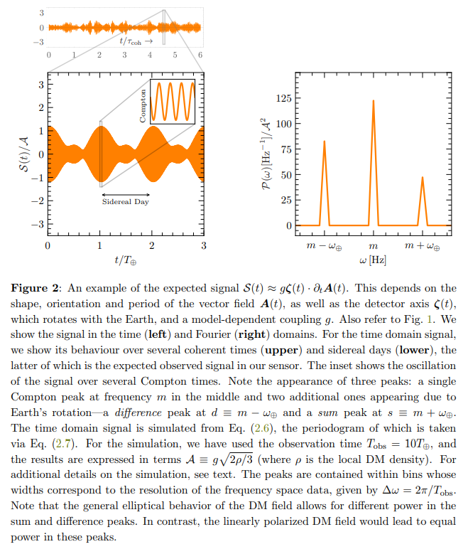
\ Fig. 2 shows an example of a signal in the short observation time regime, in both the time (Eq. (2.6)) and Fourier (Eq. (2.9)) domain. To generate them, we have taken A = 1 [A], m = 2π Hz, ϕ = 45◦ , Tobs = 10T⊕, and, for the purposes of fast convergence, T⊕ = 100 s. Here, [A] are the units of A, which depend on the quantity being measured by the experiment. We have also taken α ≡ (αx, αy, αz) ⊺ = (1, 0.7, 0.2)⊺ and φ ≡ (φx, φy, φz) ⊺ = (π/2, π/4, π/3)⊺ . When running our future simulations, we sample these six variables independently from their respective distributions.
\ There are three characteristic timescales within the signal: the Compton scale, the Earth’s rotation period, and the coherent (de Broglie) scale. The first two of these are present in the larger panels of Fig. 2. The Earth’s rotation period is evident from the time domain signal, which we have shown for three full rotation periods. The Compton scale is much faster than this scale (see inset), making the signal appear solid in shape. Crucially, we see that the vector ULDM field leaves a characteristic three-peak signal in the Fourier domain[5]. One peak is present at the Compton frequency ω = m, which previous frequency-space analyses have focused on [36, 38]. However, a further two peaks manifest as a result of the Earth’s rotation, which are spaced ω⊕ away from the Compton peak. These additional peaks, the use of which has been ignored in previous accelerometer analyses[6], only appear as Tobs ≥ T⊕; shorter observation times do not give us enough resolution in the frequency domain to resolve them[7]. We call the peak at the Compton frequency the Compton peak, that at s the sum peak, and that at d the difference peak.
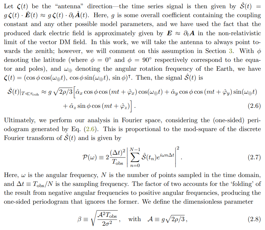
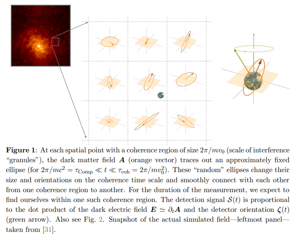
\ We argued earlier that, within a coherence patch, we expect the vector field to undergo an elliptical motion with period 2π/m (see Fig. 1), as opposed to a linear one commonly used in the literature. In both the linear and elliptical cases, the time domain signal, S(t), is sinusoidal and contains the angular frequencies m and m ± ω⊕. Repeating the analysis of [40] in the time domain, but without the linear polarization assumption, we expect qualitatively similar results (with more statistical spread on the time averaged power). However, there are some important differences when analysing the expected signal in Fourier space.
\ In the elliptical case, the power contained in the m and m ± ω⊕ peaks is statistically uncorrelated (see Appendix C). On the other hand, for the linear polarization case, the power at m and m±ω⊕ is correlated, with equal power in the sum and difference peaks. This can be seen by noting that, in this case, all the components of the vector are in phase. The statistical independence in the elliptical case significantly simplifies our analysis pipeline for projected sensitivities. Furthermore, the distinction in power at m±ω⊕ is also relevant in case of a detection since we would expect different powers in the elliptical case.
\
:::info This paper is available on arxiv under CC BY 4.0 DEED license.
:::
[5] Such a signal would also be seen in the case of the gradient of a scalar field, as mentioned in Ref. [45], and its form is similar to that of Eq. (2.6). See Appendix D for details.
\ [6] Ref. [36] also noted this spectral splitting; however, the focus was on the Compton peak for the purposes of that analysis. In Ref. [67], this splitting as it relates to a global network of magnetometers was used.
\ [7] For us, the observation time is defined as the amount of time that data are continuously taken. As such, the total expedition time of the entire experiment is equivalent to Tobs.
This content originally appeared on HackerNoon and was authored by Phenomenology Technology
Phenomenology Technology | Sciencx (2024-10-27T21:21:55+00:00) The Dark Matter Detector Signal. Retrieved from https://www.scien.cx/2024/10/27/the-dark-matter-detector-signal/
Please log in to upload a file.
There are no updates yet.
Click the Upload button above to add an update.
