This content originally appeared on HackerNoon and was authored by Hyper Inflation
:::info Author:
(1) Laurence Francis Lacey, Lacey Solutions Ltd, Skerries, County Dublin, Ireland.
:::
:::tip Editor's Note: This is Part 4 of 7 of a study on how changes in the money supply, economic growth, and savings levels affect inflation. Read the rest below.
:::
Table of Links
- Abstract and 1 Introduction
- 2. Methods
- 2.1 Statistical Methodology
- 2.2 US Time Series Data
- 2.3 Hyperinflation Model
- 3. Results
- 3.1 Characterisation of Price Inflation
- 3.2 Characterisation of Hyperinflation in the Weimar Republic (1922 to 1923)
- 4. Discussion
- 5. Conclusion, Supplementary materials, Acknowledgements, and References
- Appendix
3.1 Characterisation of Price Inflation
A plot of the natural log-transformed US BMS time series over the period 2001 to 2019 is given in Figure 1. The year 2001 is the reference year (time = 0), and the BMS data were expressed relative to the value obtained in year 2001. The corresponding plots for the natural log-transformed US CPI time series is given in Figure 2; the natural log-transformed US real GDP time series is given in Figure 3; the natural log-transformed average American household savings time series is given in Figure 4
\
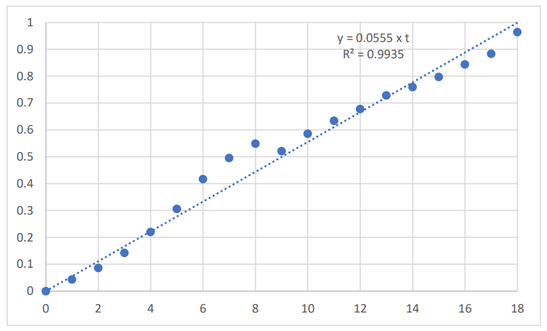
\ The average annual rate of growth of the US BMS, over the period 2001 to 2019, was 5.7%, with:
\
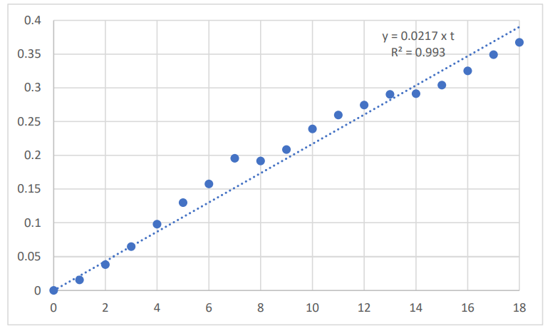
\ The average annual rate of US price inflation as measured by CPI, over the period 2001 to 2019, was 2.2%, with:
\ 𝑣𝐶𝑃𝐼(𝑡) = 0.0217 x t
\
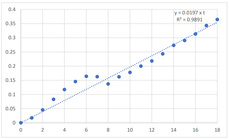
\ The average annual rate of growth of the US real GDP, over the period 2001 to 2019, was 2.0%, with:
\ 𝑣𝐺𝐷𝑃(𝑡) = 0.0197 x t
\
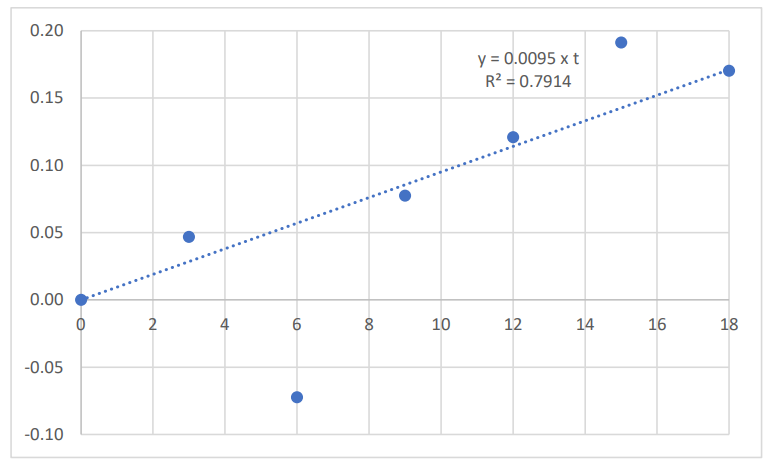
\ The average annual rate of growth of American household savings, over the period 2001 to 2019, was 1.0%, with:
\ 𝑣𝑆𝐴𝑉(𝑡) = 0.0095 x t
\ The linear regression fits are summarised in Table 1.
\
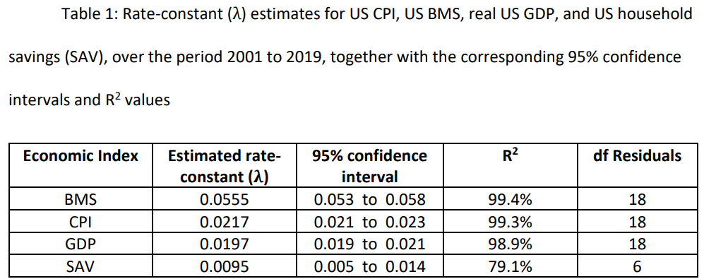
\ BMS, broad money supply; CPI, consumer price index; GDP, (real) gross domestic product; SAV, average American household savings; df, degrees of freedom
\ Henceforth, the annual US household savings estimates for the years not available were imputed, using the regression fit obtained from the available years of data.
\ The residual time series (RES(t)) was obtained from the relationship:
\ 𝑅𝐸𝑆(𝑡) = 𝑣𝐵𝑀𝑆(𝑡) − 𝑣𝐺𝐷𝑃(𝑡) − 𝑣𝑆𝐴𝑉(𝑡) − 𝑣𝐶𝑃𝐼
\ This residual time series is plotted in Figure 5.
\
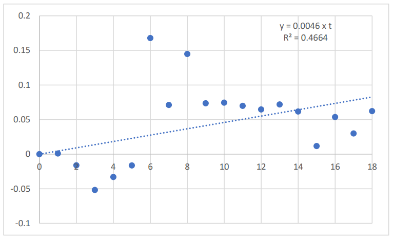
\ The average annual rate of growth of the residual time series (RES(t)), over the period 2001 to 2019, was 0.5%, with:
\ 𝑅𝐸𝑆(𝑡) = 0.0046 x t
\ This gives:
\ 𝑣𝐶𝑃𝐼(𝑡) = 𝑣𝐵𝑀𝑆(𝑡) − 𝑣𝐺𝐷𝑃(𝑡) − 𝑣𝑆𝐴𝑉(𝑡) − 𝑅𝐸𝑆(𝑡)
\ Further detail of the residual time series (RES(t)), over the period 2001 to 2019, are given in Table 2.
\

\ RES, residual time series; df, degrees of freedom
\
:::info This paper is available on arxiv under CC BY-NC-ND 4.0 DEED license.
:::
\
This content originally appeared on HackerNoon and was authored by Hyper Inflation
Hyper Inflation | Sciencx (2025-01-02T07:30:11+00:00) The Characteristics of Price Inflation. Retrieved from https://www.scien.cx/2025/01/02/the-characteristics-of-price-inflation/
Please log in to upload a file.
There are no updates yet.
Click the Upload button above to add an update.
