K-nearest neighbors algorithm detailed in Python

The K Nearest Neighbor algorithm was one of the first algorithms to determine a solution for finding the best route between multiple cities. This algorithm quickly generates a shorter path between two points and is considered the most straightforward algorithm for sorting tasks in supervised learning.

Jupyter Notebook

See The Jupyter Notebook for the concepts we’ll cover on building machine learning models and my LinkedIn Profile for other Data Science articles and tutorials.

KNN is used to sort objects based on training examples closest to the characteristic space in the variable area in our dataset. To use KNN, it is necessary to:

  • Training data;
  • Set the metric for distance calculation;
  • Set the value of K (number of closest neighbors that the algorithm will consider).

The process of calculating an unknown example with the KNN algorithm consists of calculating the distance between a strange example and the other models in the training set to identify the nearest neighbor; that is, we use the class label of the nearest neighbors to determine the class label of the unfamiliar example.

Therefore, the sorting process with the KNN algorithm is accomplished by determining the unknown sample class from the list of nearest neighbors. One of the critical points of the KNN model is to set precisely the value of K.

There are several different ways to calculate this distance, the Euclidean distance being one of the simplest. We have the distance between p and q, that is, two points, and we go squared to the value to use the absolute value.

Distance Metrics

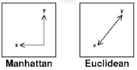
We can influence the outcome of our model by changing the distance metric. Other ways to measure distance:

  • Manhattan
  • Minkowsky
  • Hamming

Normalization

For the application of the KNN algorithm, we must normalize the data first of all. Distance measurements are susceptible to the scale of the data, and for this reason, we should normalize the data before applying the algorithm and build the predictive model. So, if we have data points with very different scales, when we calculate the distance with the Euclidean form, we will have very discrepant values — we should put the data on the same scale.

Voronoi Cell Structure

Now that we have a general idea of what KNN is, we’ll go into the more technical details of the algorithm to understand the structure of Voronoi cells.

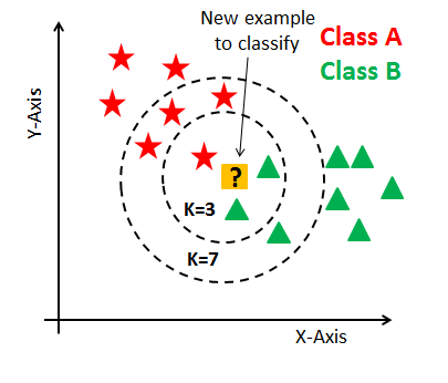
We have a plot with two classes: green triangles and red stars. The question is, which of the two groups does the yellow interrogation belong to? Intuitively, the data point in the yellow square belongs to the group of triangles by its proximity to two triangles, and this point likely has the same characteristics as a triangle.

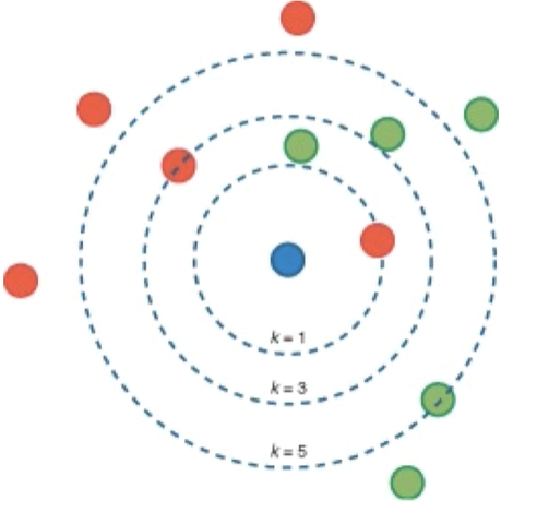
In practice, this is what the KNN algorithm does. The nearest neighbor sorts the data point by calculating the distance from this new data point to the nearest neighbors — the K parameter we use as the hyperparameter of the KNN algorithm defines how many closer neighbors it fetches the distance calculation.

For example, if we use a value equal to 3, the KNN will compare the new data point with the three closest neighbors in each class and then take a vote. Generally speaking, there are some mathematical calculations so that the algorithm can choose in which category to define each new data point and thus sort each point in our training dataset.

Voronoi Polygon

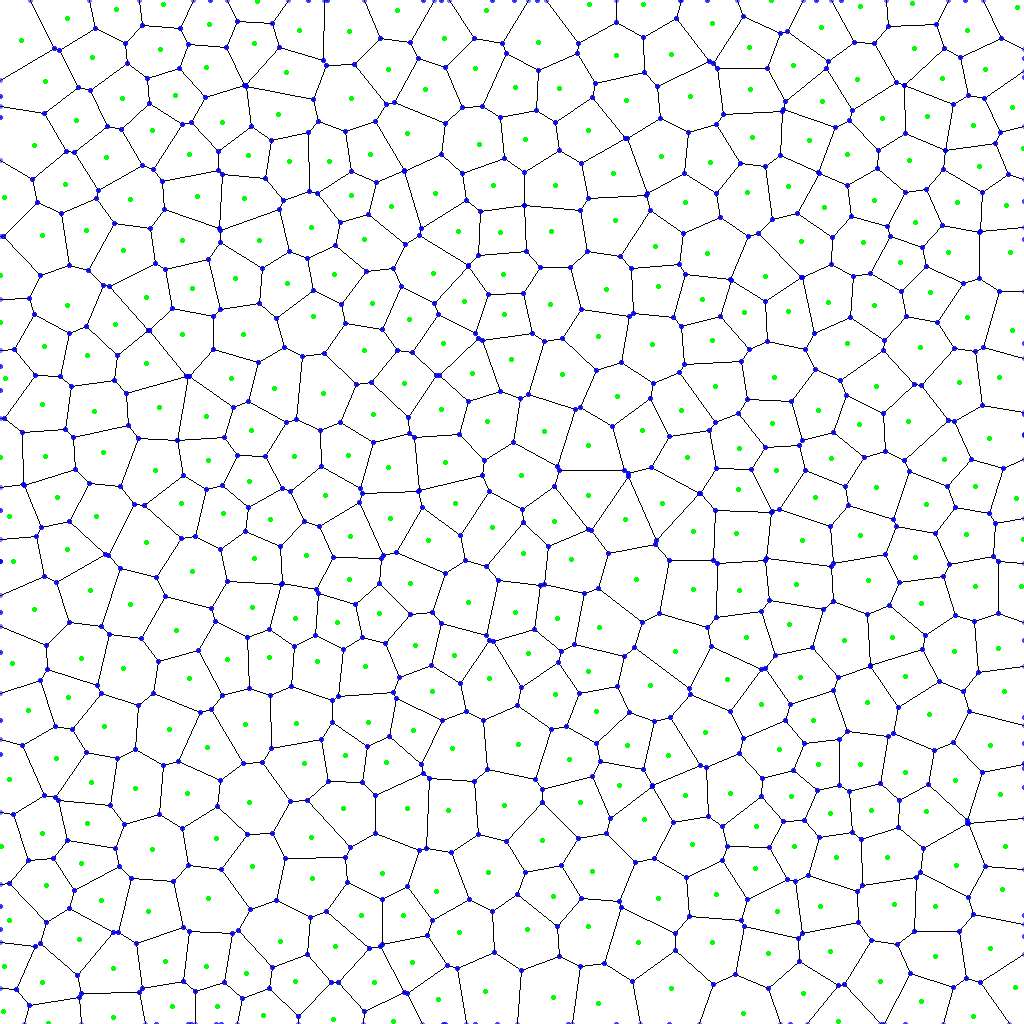
Let’s assume that the new data point, represented by the red square, belongs to the class of stars. The important aspect of distance measurements is that the nearest neighbor is not just a data point but a region; that is, the data points in a given area will belong to the respective star class.

This region is called the Voronoi cell, a polygon with straight lines when the Euclidean distance measures distance. Therefore, the calculation is not done for each data point or between specific data points but for a region where the data points are.

The size of each cell is determined by the number of examples available in the training dataset. For each training instance in which the Voronoi cell is computed, we see an area representing partitions in the data space and without overlap. Typically, each region has a single data point, and all of this is done with mathematical calculations implemented in the algorithm.

Voronoi Cell Structure

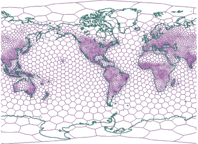
The space of characteristics and attributes is divided into more manageable areas such as honeycombs. This subdivision is known as the Voronoi arrangement. The data structure that describes it is the Voronoi cell structure. The interior of each cell consists of all the points closest to a specific convex interlacing point.

Voronoi cell structures tend to be irregularly shaped polygons. We can adjust the number and location of cells to match the density and area of the data within the dataset.

For example, a Voronoi cell structure can subdivide the earth into polygons based on the human population. The population is dense, there are small polygons, and the population is sparse; there are large polygons — the Voronoi diagram is widely used in computational geometry.

How does KNN work?

From a training data set, where X represents the predictor variables, and Y represents the target variable so that the classification of a new data point occurs, the following steps are performed for a KNN algorithm:

  1. The distance is computed between X and Xi for each Xi value;
  2. The nearest k-neighbor Xin and its respective class are chosen;
  3. Returns the most frequent y value in list yi1, yi2, … Yin.

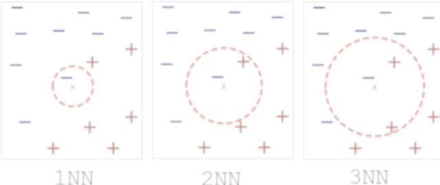
In addition to impacting the KNN performance model, the value of K will define the success or failure of a model created with this algorithm. If the K value is too high, the KNN algorithm can result in a model with low accuracy; if the K value is too low, the model is susceptible to outliers and may generate incorrect ratings.

The goal is to define the K value that manages the most generalizable model possible — the primary purpose for any Machine Learning. As we change the value of K, the same data point X belongs to another class, and to estimate the class of a new X pattern, the KNN algorithm calculates the nearest neighboring K to X.

Distance Measurements

There are several measures of distances, the primary purpose of these measures is to identify similar data. Just like the K value, the distance measurement directly influences the performance of models created with KNN.

The Euclidean distance is the default option for numerical attributes, that is, numerical variables. Space is measured with the formula below:

The Euclidean distance is symmetrical and treats all dimensions equally. One of the downsides of this measure is its sensitivity to outliers values, and for that reason, we have to do a little more to pre-process the data before delivering it to the KNN algorithm.

Manhattan and Euclidean distances are the most commonly used in KNN algorithms.

The accuracy of the classification using the KNN algorithm depends heavily on the data model. Most of the time, attributes need to be normalized to prevent distance measurements from being dominated by a single feature.

KNN differential

The KNN uses the Parameter K, which indicates the number of neighbors used by the algorithm during the training phase.

The K parameter causes the algorithm to achieve a more refined classification. Still, the optimal value of K varies from one problem to another, which means that we have to test different K values for each situation we are working on.

Business Problem

KNN classification is one of the simplest algorithms for Machine Learning; being a lazy algorithm; no computation is performed in the dataset until a new data point is tested.

That is, it does not perform all processing at once as in regression models. With KNN, the behavior is slightly different. KNN creates a comparison table with the distances it calculates. Therefore, when we have a new data point, the algorithm queries that table and checks where to sort the latest data point.

We will make handwritten digit predictions in the mnist dataset. This is an example of multiclass classification because our model will predict one out of 10 possible outputs for each record (digits 0 through 10).

When we have the prediction of only two possible outputs, the classification is binary. When we have more than two classes to predict, we call it multiclass classification — the processing of the data is practically the same; the difference is that we now have more categories that we can predict.

Dataset

We can load the dataset we’re going to work on with the load_digits the package datasets of the sklearn library. Therefore, we already have the dataset within the scikit-learn library itself.

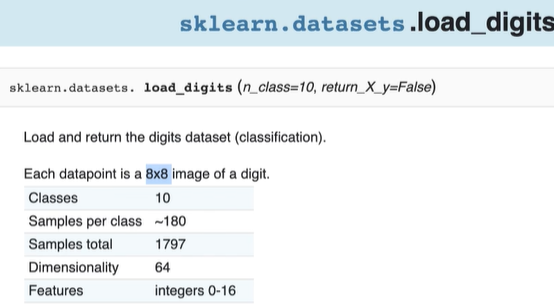
Each data point is an 8×8 image of a digit, that is, 8 pixels high and 8 pixels wide — every image is an array of pixels, in other words, a mathematical element. In this dataset, we have ten possible classes (digits 0 through 10), approximately 180 examples per class and a total of 1797 records, and 64 variables that correspond to 1 pixel.

from IPython.display import Image
Image('image/digits.png')
# Each pixel is a variable
from IPython.display import Image
Image('image/flatten.png')

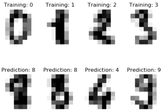
The image is an array, that is, a two-dimensional object. However, we cannot feed the model directly with the matrix, so we transform the two-dimensional object (matrix) into a one-dimensional object (vector).

Therefore, we take the first line of the matrix and place it in the vector, move to the second line of the matrix, and concatenate to the vector again; that is, we will attach the groups next to each other until we formulate a one-dimensional object.

KNN Rating in Python — Loading and Exploring dataset

Let’s sort a set of pixels and tell you the associated type of digit from 0 to 10. Let’s start loading and exploring the dataset:

# Load packages
import numpy as np
from sklearn import datasets # Get dataset
from sklearn.metrics import confusion_matrix # confusion matrix
from sklearn.model_selection import train_test_split # split data
from sklearn.neighbors import KNeighborsClassifier # kNN algorithm
from sklearn.metrics import classification_report # rating metrics
import matplotlib.pyplot as plt
import warnings # Disable warnings
warnings.filterwarnings('ignore')
# Load dataset
digits = datasets.load_digits()
digits
{'data': array([[ 0., 0., 5., ..., 0., 0., 0.],
[ 0., 0., 0., ..., 10., 0., 0.],
[ 0., 0., 0., ..., 16., 9., 0.],
...,
[ 0., 0., 1., ..., 6., 0., 0.],
[ 0., 0., 2., ..., 12., 0., 0.],
[ 0., 0., 10., ..., 12., 1., 0.]]),
'target': array([0, 1, 2, ..., 8, 9, 8]),
'frame': None,
'feature_names': ['pixel_0_0',
'pixel_0_1',
'pixel_0_2',
'pixel_0_3',...

Next, we will print the pixels that are the input data and the classes that are the output data:

# Viewing some images and labels - Print pixels
images_e_labels = list(zip(digits.images, digits.target))
for index, (image, label) in enumerate(images_e_labels[:4]):
plt.subplot(2, 4, index + 1)
plt.axis('off')
plt.imshow(image, cmap = plt.cm.gray_r, interpolation='nearest')
plt.title('Label: %i' % label)

Therefore, we have a set of pixels representing labels 0, 1, 2, and 3. For this type of classification to be done, someone must devote themselves to labeling, which is to put the labels for the observations — usually, it is the most critical part of the process.

Some tools facilitate this labeling process, but this is a more artificial intelligence-oriented issue.

Here we separate what represents the input data and what the output data represents:

# Generate X and Y
X = digits.data
Y = digits.target
# X and Y format
print(X.shape, Y.shape)
(1797, 64) (1797,)

For X, we have 1797 representing the pixels of a digit and 64 columns because each pixel is a variable (each “square” of the vector). So, we have an 8×8 image, a matrix diluted in vector, and now we have each item “square” of the vector is configured as a variable.

Data Preprocessing

Here we need to apply normalization because KNN works best when data is normalized.

The first thing to do here is to split the data into training and test datasets. We passed as input of the function the X and Y sets defined just above; we indicate the test_size size of 30% to put the records into the test and the other 70% in the training dataset.

This function works randomly, so each run, the training, and test data will be completely random. So that we can reproduce the same results when we run The Jupyter Notebook, we apply the random_state.

# Splitting into training and test data
X_train, testData, Y_train, testLabels = train_test_split(X, Y, test_size = 0.30, random_state = 101)

We wrote the 4 function results to X_train, testData, y_train, testLabels. Therefore, we divided between training data and test data.

Now, optionally, an excellent alternative to increase the model’s accuracy is to validate during training, a kind of performance evaluation during the algorithm’s training. Typically, this helps you make decisions during your own training:

trainData, validData, trainLabels, validLabels = train_test_split(X_train,                                                y_train, test_size = 0.1,                                                               random_state = 84)

So, we took the training data and did a new split for validation. In practice, we will have 3 sets of data: training, testing, and validation that will contain 10% of the dataset to evaluate the model during training.

# Printing the number of examples (notes) on each dataset
print("Training Examples: {}".format(len(trainLabels)))
print("Validation Examples: {}".format(len(validLabels)))
print("Test Examples: {}".format(len(testLabels)))
Training Examples: 1131
Validation Examples: 126
Test Examples: 540

A widespread division uses 70% for training, 20% for testing, and 10% validation.

Apply normalization

For each of the values, we have different scales. Because the KNN algorithm calculates the mathematical distance, it works best when we normalize the data, that is, but the data on the same scale.

# Normalization of data by Average
# Calculation of the average of the training dataset
X_norm = np.mean(X, axis = 0)
# Normalization of training and test data
X_train_norm = trainData - X_norm
X_valid_norm = validData - X_norm
X_test_norm = testData - X_norm

Above we apply the calculation of the average of all values of our input data set X. It is unnecessary to normalize Y because it represents a class from 0 to 10; that is, this data is already on a single scale, or rather, they are just categories.

print(X_train_norm.shape, X_valid_norm.shape, X_test_norm.shape)
(1131, 64) (126, 64) (540, 64)

Above, we have the shapes of the 3 training, validation, and test sets with the same number of attributes. What will change from one group to another is just the number of observations (lines).

KNN Rating in Python — Testing the Best K Value

One of the main parameters for KNN is the K value itself, which represents the number of closest neighbors that the algorithm will use to do the distance calculation.

Here below, we will define a range of K values to test:

# Range of k values that we will test
kVals = range(1, 30, 2)

We have an infinite value for K. In this case; we use the range function in Python to create a range of 15 elements, where we start with the value 1 and go up to the number 30 (exclusive) and jumping from 2 to 2, that is, we select only the odd values that present the best result with KNN.

In practice, the algorithm does not look at a unique data point but rather a Voronoi polygon and, based on this, will make the distance calculation. With even values, we may have the problem of the tie in the KNN vote.

# Empty list to receive accuracy
accuracy = []

Above, we create an empty list to receive the accuracy.

# Loop on all k values to test each of them
for k in kVals:

# Loop on all k values to test each of them
modelKNN = KNeighborsClassifier(n_neighbors = k)
modelKNN.fit(trainData, trainLabels)

We create a for loop for the K values, where we will select each K value in kVals, the range of odd numbers. Next, we create a KNN model with the KNeighborsClassifier and pass the K parameter for the neighbors. In the end, we trained the model; that is, we created the KNN with different K values, and we will evaluate which K value granted the best performance.

Best Value of K

Below we do the validation using the validation set during the training and print the K values with their respective accuracy:

# Evaluating the model and updating the list of accuracys
score = modelKNN.score(validData, validLabels)
print("With a value of k = %d, accuracy is = %.2f%%"% (k, score * 100))
accuracy.append(score)
With a value of k = 1, accuracy is = 99.21%
With a value of k = 3, accuracy is = 100.00%
With a value of k = 5, accuracy is = 100.00%
With a value of k = 7, accuracy is = 99.21%
With a value of k = 9, accuracy is = 98.41%
With a value of k = 11, accuracy is = 98.41%
With a value of k = 13, accuracy is = 97.62%
With a value of k = 15, accuracy is = 97.62%
With a value of k = 17, accuracy is = 97.62%
With a value of k = 19, accuracy is = 97.62%
With a value of k = 21, accuracy is = 97.62%
With a value of k = 23, accuracy is = 97.62%
With a value of k = 25, accuracy is = 96.83%
With a value of k = 27, accuracy is = 96.83%
With a value of k = 29, accuracy is = 96.83%

Clearly, the value of K at 3 or 5 has better performance. To reach this conclusion, we use the validation set.

Now to get the best value, let’s use NumPy’s argmax function. This function picks up exactly the maximum value considering all the accuracy levels of the numeric values.

# Getting the value of k that presented the highest accuracy
i = np.argmax(accuracy)
print("The value of k = %d reached the highest accuracy of %.2f%% in the validation data!" % (kVals[i],
accuracy[i] * 100))
The value of k = 3 reached the highest accuracy of 100.00% in the validation data!
KNN Classification in Python - KNN Model Construction and Training

Finally, we have that the value of K = 3 is the one that presents the best result in the validation data. Based on this, we can now create the final version of the model using K = 3.

Create KNN template

# Creating the model final version model with the highest value of k
finalModel = KNeighborsClassifier(n_neighbors = kVals[i])

Above, we put kVals in index “i” representing the best value within the Set of K that we have already tested above. We chose to use kVals[i] instead of 3 to automate the code, and it would be enough to change the value to the range of kVals freely. Rotated the code above, we have the KNN model created!

Train Model KNN

The method used by the algorithm was that of Minkowski. Within scikit-learn, the algorithm is using Minkowski as a mathematical distance measure.

# Model training
finalModel.fit(trainData, trainLabels)

After the model training, we will make the performance evaluation; we present the model data that he has not yet seen.

During the training, the model had access to the training data to learn the relationships. Now new data will be presented to the model to verify if the model is generalizable.

Make Predictions

We will make predictions with the test data and then evaluate your performance. We used the validation data exclusively during the search for the best K value.

# Predictions with test data
predictions = finalModel.predict(testData)

We call the predict function for the finalModel object; the model created just above. As a parameter, we pass testData and record all of this in the predictions object.

When printing the summary, we have the metrics of precision, recall, f1, and support. Each metric helps us understand the evaluation of the model from a different perspective. Generally, precision is the most objective metric — the model has reached almost 100% accuracy. This explains that the data set is well organized, the problem is relatively simple, and we find the ideal value of K.

# Model performance in test data
print("Model Evaluation in Test Data")
print(classification_report(testLabels, predictions))
Model Evaluation in Test Data
precision recall f1-score support
           0       1.00      1.00      1.00        53
1 0.95 0.98 0.96 55
2 1.00 1.00 1.00 49
3 0.98 0.98 0.98 54
4 1.00 0.98 0.99 61
5 0.98 1.00 0.99 59
6 1.00 0.98 0.99 46
7 1.00 1.00 1.00 56
8 1.00 0.95 0.97 59
9 0.96 1.00 0.98 48
    accuracy                           0.99       540
macro avg 0.99 0.99 0.99 540
weighted avg 0.99 0.99 0.99 540

Another thing we can do to evaluate the performance of the model is to draw a confusion matrix. We use the confusion_matrix function and pass two parameters: testLabels and predictions; that is, we will compare the historical observed data and predictions of the model created just now.

# Confusion Matrix of the Final Model
print ("Confusion matrix")
print(confusion_matrix(testLabels, predictions))
Confusion matrix
[[53 0 0 0 0 0 0 0 0 0]
[ 0 54 0 0 0 1 0 0 0 0]
[ 0 0 49 0 0 0 0 0 0 0]
[ 0 0 0 53 0 0 0 0 0 1]
[ 0 0 0 0 60 0 0 0 0 1]
[ 0 0 0 0 0 59 0 0 0 0]
[ 0 1 0 0 0 0 45 0 0 0]
[ 0 0 0 0 0 0 0 56 0 0]
[ 0 2 0 1 0 0 0 0 56 0]
[ 0 0 0 0 0 0 0 0 0 48]]

The function’s output is a multiclass confusion matrix; we have the 10 digits from 0 to 10 of the observed values and the other 10 digits of the predicted values.

Looking at the first column, when the observed value was 0, and the predicted value was 0, 0 models hit 53 times — the model hit all predictions.

Looking at the second column, when the observed value was 1, the predicted value was 9 and 7, so the model ended up making some mistakes at some point — the confusion matrix helps us to observe it more clearly.

Random Data Predictions

Now we make predictions with random data from the test dataset. Below we have a loop where we will get random values from the testLabels; we do not know which value to take.

For each “i” value in the random set that returns, we will take an element (digit) and place it in the image object, and through that object, we make a prediction. After the forecast, we will adjust the shape and print on the screen:

# Making predictions with the trained model using test data
for i in np.random.randint(0, high=len(testLabels), size=(2,)):

# Gets an image and makes the prediction
image = testData[i]
prediction = finalModel.predict([image])[0]

# Show predictions
imgdata = np.array(image, dtype='float')
pixels = imgdata.reshape((8,8))
plt.imshow(pixels,cmap='gray')
plt.annotate(prediction,(3,3),bbox={'facecolor':'white'},fontsize=16)
print("I believe this digit is: {}".format(prediction))
plt.show()
I believe this digit is: 3
I believe this digit is: 9

If we are already satisfied with the result of the model, we can use it to meet the ultimate purpose of making new predictions.

KNN Classification in Python — Predictions on New Data with the Trained Model

After we train the model and evaluate its performance, we can use the model to make predictions with new data — in this case; it is intended to make digit predictions.

Below is a list that represents the pixels of a digit from 0 to 10. We have the 64 variables where each position is a pixel of any digit — the digit is an image in a two-dimensional matrix converted into a vector.

# Setting a new digit (input data)
newDigit = [0., 0., 0., 8., 15., 1., 0., 0., 0., 0., 0., 12., 14., 0., 0., 0., 0., 0., 3., 16., 7., 0., 0., 0., 0., 0., 6., 16., 2., 0., 0., 0., 0., 0., 7., 16., 16., 13., 5., 0., 0., 0., 15., 16., 9., 9., 14., 0., 0., 0., 3., 14., 9., 2., 16., 2., 0., 0., 0., 7., 15., 16., 11., 0.]

Next, we need to normalize the data since the model learned from normalized data.

# Normalizing the new digit
newDigit_norm = newDigit - X_norm

We pass the normalized digit as a parameter for finalModel prediction:

# Making the prediction with the trained model
newPrediction = finalModel.predict([newDigit_norm])

Below we take the pixels, put them back in a two-dimensional matrix format, adjust the scale, and print:

# Model prediction
imgdata = np.array(newDigit, dtype='float')
pixels = imgdata.reshape((8,8))
plt.imshow(pixels, cmap='gray')
plt.annotate(newPrediction,(3,3), bbox={'facecolor':'white'},fontsize=16)
print("I believe this digit is: {}".format(newPrediction))
plt.show()
I believe this digit is: [6]

And there we have it. Our model is working. With this, we complete the KNN model for digit predictions. I hope you have found this helpful. Thank you for reading. ?


K-nearest neighbors algorithm detailed in Python was originally published in Level Up Coding on Medium, where people are continuing the conversation by highlighting and responding to this story.


This content originally appeared on Level Up Coding - Medium and was authored by Anello

The K Nearest Neighbor algorithm was one of the first algorithms to determine a solution for finding the best route between multiple cities. This algorithm quickly generates a shorter path between two points and is considered the most straightforward algorithm for sorting tasks in supervised learning.

Jupyter Notebook

See The Jupyter Notebook for the concepts we’ll cover on building machine learning models and my LinkedIn Profile for other Data Science articles and tutorials.

KNN is used to sort objects based on training examples closest to the characteristic space in the variable area in our dataset. To use KNN, it is necessary to:

  • Training data;
  • Set the metric for distance calculation;
  • Set the value of K (number of closest neighbors that the algorithm will consider).

The process of calculating an unknown example with the KNN algorithm consists of calculating the distance between a strange example and the other models in the training set to identify the nearest neighbor; that is, we use the class label of the nearest neighbors to determine the class label of the unfamiliar example.

Therefore, the sorting process with the KNN algorithm is accomplished by determining the unknown sample class from the list of nearest neighbors. One of the critical points of the KNN model is to set precisely the value of K.

There are several different ways to calculate this distance, the Euclidean distance being one of the simplest. We have the distance between p and q, that is, two points, and we go squared to the value to use the absolute value.

Distance Metrics

We can influence the outcome of our model by changing the distance metric. Other ways to measure distance:

  • Manhattan
  • Minkowsky
  • Hamming

Normalization

For the application of the KNN algorithm, we must normalize the data first of all. Distance measurements are susceptible to the scale of the data, and for this reason, we should normalize the data before applying the algorithm and build the predictive model. So, if we have data points with very different scales, when we calculate the distance with the Euclidean form, we will have very discrepant values — we should put the data on the same scale.

Voronoi Cell Structure

Now that we have a general idea of what KNN is, we’ll go into the more technical details of the algorithm to understand the structure of Voronoi cells.
We have a plot with two classes: green triangles and red stars. The question is, which of the two groups does the yellow interrogation belong to? Intuitively, the data point in the yellow square belongs to the group of triangles by its proximity to two triangles, and this point likely has the same characteristics as a triangle.

In practice, this is what the KNN algorithm does. The nearest neighbor sorts the data point by calculating the distance from this new data point to the nearest neighbors — the K parameter we use as the hyperparameter of the KNN algorithm defines how many closer neighbors it fetches the distance calculation.

For example, if we use a value equal to 3, the KNN will compare the new data point with the three closest neighbors in each class and then take a vote. Generally speaking, there are some mathematical calculations so that the algorithm can choose in which category to define each new data point and thus sort each point in our training dataset.
Voronoi Polygon

Let’s assume that the new data point, represented by the red square, belongs to the class of stars. The important aspect of distance measurements is that the nearest neighbor is not just a data point but a region; that is, the data points in a given area will belong to the respective star class.

This region is called the Voronoi cell, a polygon with straight lines when the Euclidean distance measures distance. Therefore, the calculation is not done for each data point or between specific data points but for a region where the data points are.

The size of each cell is determined by the number of examples available in the training dataset. For each training instance in which the Voronoi cell is computed, we see an area representing partitions in the data space and without overlap. Typically, each region has a single data point, and all of this is done with mathematical calculations implemented in the algorithm.

Voronoi Cell Structure
The space of characteristics and attributes is divided into more manageable areas such as honeycombs. This subdivision is known as the Voronoi arrangement. The data structure that describes it is the Voronoi cell structure. The interior of each cell consists of all the points closest to a specific convex interlacing point.

Voronoi cell structures tend to be irregularly shaped polygons. We can adjust the number and location of cells to match the density and area of the data within the dataset.

For example, a Voronoi cell structure can subdivide the earth into polygons based on the human population. The population is dense, there are small polygons, and the population is sparse; there are large polygons — the Voronoi diagram is widely used in computational geometry.

How does KNN work?

From a training data set, where X represents the predictor variables, and Y represents the target variable so that the classification of a new data point occurs, the following steps are performed for a KNN algorithm:

  1. The distance is computed between X and Xi for each Xi value;
  2. The nearest k-neighbor Xin and its respective class are chosen;
  3. Returns the most frequent y value in list yi1, yi2, … Yin.

In addition to impacting the KNN performance model, the value of K will define the success or failure of a model created with this algorithm. If the K value is too high, the KNN algorithm can result in a model with low accuracy; if the K value is too low, the model is susceptible to outliers and may generate incorrect ratings.
The goal is to define the K value that manages the most generalizable model possible — the primary purpose for any Machine Learning. As we change the value of K, the same data point X belongs to another class, and to estimate the class of a new X pattern, the KNN algorithm calculates the nearest neighboring K to X.

Distance Measurements

There are several measures of distances, the primary purpose of these measures is to identify similar data. Just like the K value, the distance measurement directly influences the performance of models created with KNN.

The Euclidean distance is the default option for numerical attributes, that is, numerical variables. Space is measured with the formula below:

The Euclidean distance is symmetrical and treats all dimensions equally. One of the downsides of this measure is its sensitivity to outliers values, and for that reason, we have to do a little more to pre-process the data before delivering it to the KNN algorithm.

Manhattan and Euclidean distances are the most commonly used in KNN algorithms.
The accuracy of the classification using the KNN algorithm depends heavily on the data model. Most of the time, attributes need to be normalized to prevent distance measurements from being dominated by a single feature.

KNN differential

The KNN uses the Parameter K, which indicates the number of neighbors used by the algorithm during the training phase.
The K parameter causes the algorithm to achieve a more refined classification. Still, the optimal value of K varies from one problem to another, which means that we have to test different K values for each situation we are working on.

Business Problem

KNN classification is one of the simplest algorithms for Machine Learning; being a lazy algorithm; no computation is performed in the dataset until a new data point is tested.

That is, it does not perform all processing at once as in regression models. With KNN, the behavior is slightly different. KNN creates a comparison table with the distances it calculates. Therefore, when we have a new data point, the algorithm queries that table and checks where to sort the latest data point.

We will make handwritten digit predictions in the mnist dataset. This is an example of multiclass classification because our model will predict one out of 10 possible outputs for each record (digits 0 through 10).

When we have the prediction of only two possible outputs, the classification is binary. When we have more than two classes to predict, we call it multiclass classification — the processing of the data is practically the same; the difference is that we now have more categories that we can predict.

Dataset

We can load the dataset we’re going to work on with the load_digits the package datasets of the sklearn library. Therefore, we already have the dataset within the scikit-learn library itself.
Each data point is an 8x8 image of a digit, that is, 8 pixels high and 8 pixels wide — every image is an array of pixels, in other words, a mathematical element. In this dataset, we have ten possible classes (digits 0 through 10), approximately 180 examples per class and a total of 1797 records, and 64 variables that correspond to 1 pixel.

from IPython.display import Image
Image('image/digits.png')
# Each pixel is a variable
from IPython.display import Image
Image('image/flatten.png')
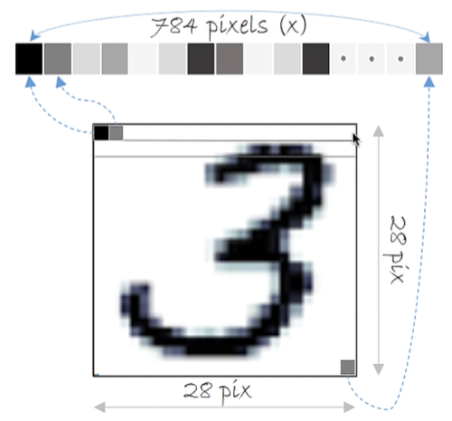
The image is an array, that is, a two-dimensional object. However, we cannot feed the model directly with the matrix, so we transform the two-dimensional object (matrix) into a one-dimensional object (vector).

Therefore, we take the first line of the matrix and place it in the vector, move to the second line of the matrix, and concatenate to the vector again; that is, we will attach the groups next to each other until we formulate a one-dimensional object.

KNN Rating in Python — Loading and Exploring dataset

Let’s sort a set of pixels and tell you the associated type of digit from 0 to 10. Let’s start loading and exploring the dataset:

# Load packages
import numpy as np
from sklearn import datasets # Get dataset
from sklearn.metrics import confusion_matrix # confusion matrix
from sklearn.model_selection import train_test_split # split data
from sklearn.neighbors import KNeighborsClassifier # kNN algorithm
from sklearn.metrics import classification_report # rating metrics
import matplotlib.pyplot as plt
import warnings # Disable warnings
warnings.filterwarnings('ignore')
# Load dataset
digits = datasets.load_digits()
digits
{'data': array([[ 0., 0., 5., ..., 0., 0., 0.],
[ 0., 0., 0., ..., 10., 0., 0.],
[ 0., 0., 0., ..., 16., 9., 0.],
...,
[ 0., 0., 1., ..., 6., 0., 0.],
[ 0., 0., 2., ..., 12., 0., 0.],
[ 0., 0., 10., ..., 12., 1., 0.]]),
'target': array([0, 1, 2, ..., 8, 9, 8]),
'frame': None,
'feature_names': ['pixel_0_0',
'pixel_0_1',
'pixel_0_2',
'pixel_0_3',...

Next, we will print the pixels that are the input data and the classes that are the output data:

# Viewing some images and labels - Print pixels
images_e_labels = list(zip(digits.images, digits.target))
for index, (image, label) in enumerate(images_e_labels[:4]):
plt.subplot(2, 4, index + 1)
plt.axis('off')
plt.imshow(image, cmap = plt.cm.gray_r, interpolation='nearest')
plt.title('Label: %i' % label)

Therefore, we have a set of pixels representing labels 0, 1, 2, and 3. For this type of classification to be done, someone must devote themselves to labeling, which is to put the labels for the observations — usually, it is the most critical part of the process.

Some tools facilitate this labeling process, but this is a more artificial intelligence-oriented issue.

Here we separate what represents the input data and what the output data represents:

# Generate X and Y
X = digits.data
Y = digits.target
# X and Y format
print(X.shape, Y.shape)
(1797, 64) (1797,)

For X, we have 1797 representing the pixels of a digit and 64 columns because each pixel is a variable (each “square” of the vector). So, we have an 8x8 image, a matrix diluted in vector, and now we have each item “square” of the vector is configured as a variable.

Data Preprocessing

Here we need to apply normalization because KNN works best when data is normalized.

The first thing to do here is to split the data into training and test datasets. We passed as input of the function the X and Y sets defined just above; we indicate the test_size size of 30% to put the records into the test and the other 70% in the training dataset.

This function works randomly, so each run, the training, and test data will be completely random. So that we can reproduce the same results when we run The Jupyter Notebook, we apply the random_state.

# Splitting into training and test data
X_train, testData, Y_train, testLabels = train_test_split(X, Y, test_size = 0.30, random_state = 101)

We wrote the 4 function results to X_train, testData, y_train, testLabels. Therefore, we divided between training data and test data.

Now, optionally, an excellent alternative to increase the model’s accuracy is to validate during training, a kind of performance evaluation during the algorithm’s training. Typically, this helps you make decisions during your own training:

trainData, validData, trainLabels, validLabels = train_test_split(X_train,                                                y_train, test_size = 0.1,                                                               random_state = 84)

So, we took the training data and did a new split for validation. In practice, we will have 3 sets of data: training, testing, and validation that will contain 10% of the dataset to evaluate the model during training.

# Printing the number of examples (notes) on each dataset
print("Training Examples: {}".format(len(trainLabels)))
print("Validation Examples: {}".format(len(validLabels)))
print("Test Examples: {}".format(len(testLabels)))
Training Examples: 1131
Validation Examples: 126
Test Examples: 540

A widespread division uses 70% for training, 20% for testing, and 10% validation.

Apply normalization

For each of the values, we have different scales. Because the KNN algorithm calculates the mathematical distance, it works best when we normalize the data, that is, but the data on the same scale.

# Normalization of data by Average
# Calculation of the average of the training dataset
X_norm = np.mean(X, axis = 0)
# Normalization of training and test data
X_train_norm = trainData - X_norm
X_valid_norm = validData - X_norm
X_test_norm = testData - X_norm

Above we apply the calculation of the average of all values of our input data set X. It is unnecessary to normalize Y because it represents a class from 0 to 10; that is, this data is already on a single scale, or rather, they are just categories.

print(X_train_norm.shape, X_valid_norm.shape, X_test_norm.shape)
(1131, 64) (126, 64) (540, 64)

Above, we have the shapes of the 3 training, validation, and test sets with the same number of attributes. What will change from one group to another is just the number of observations (lines).

KNN Rating in Python — Testing the Best K Value

One of the main parameters for KNN is the K value itself, which represents the number of closest neighbors that the algorithm will use to do the distance calculation.

Here below, we will define a range of K values to test:

# Range of k values that we will test
kVals = range(1, 30, 2)

We have an infinite value for K. In this case; we use the range function in Python to create a range of 15 elements, where we start with the value 1 and go up to the number 30 (exclusive) and jumping from 2 to 2, that is, we select only the odd values that present the best result with KNN.

In practice, the algorithm does not look at a unique data point but rather a Voronoi polygon and, based on this, will make the distance calculation. With even values, we may have the problem of the tie in the KNN vote.

# Empty list to receive accuracy
accuracy = []

Above, we create an empty list to receive the accuracy.

# Loop on all k values to test each of them
for k in kVals:

# Loop on all k values to test each of them
modelKNN = KNeighborsClassifier(n_neighbors = k)
modelKNN.fit(trainData, trainLabels)

We create a for loop for the K values, where we will select each K value in kVals, the range of odd numbers. Next, we create a KNN model with the KNeighborsClassifier and pass the K parameter for the neighbors. In the end, we trained the model; that is, we created the KNN with different K values, and we will evaluate which K value granted the best performance.

Best Value of K

Below we do the validation using the validation set during the training and print the K values with their respective accuracy:

# Evaluating the model and updating the list of accuracys
score = modelKNN.score(validData, validLabels)
print("With a value of k = %d, accuracy is = %.2f%%"% (k, score * 100))
accuracy.append(score)
With a value of k = 1, accuracy is = 99.21%
With a value of k = 3, accuracy is = 100.00%
With a value of k = 5, accuracy is = 100.00%
With a value of k = 7, accuracy is = 99.21%
With a value of k = 9, accuracy is = 98.41%
With a value of k = 11, accuracy is = 98.41%
With a value of k = 13, accuracy is = 97.62%
With a value of k = 15, accuracy is = 97.62%
With a value of k = 17, accuracy is = 97.62%
With a value of k = 19, accuracy is = 97.62%
With a value of k = 21, accuracy is = 97.62%
With a value of k = 23, accuracy is = 97.62%
With a value of k = 25, accuracy is = 96.83%
With a value of k = 27, accuracy is = 96.83%
With a value of k = 29, accuracy is = 96.83%

Clearly, the value of K at 3 or 5 has better performance. To reach this conclusion, we use the validation set.

Now to get the best value, let’s use NumPy’s argmax function. This function picks up exactly the maximum value considering all the accuracy levels of the numeric values.

# Getting the value of k that presented the highest accuracy
i = np.argmax(accuracy)
print("The value of k = %d reached the highest accuracy of %.2f%% in the validation data!" % (kVals[i],
accuracy[i] * 100))
The value of k = 3 reached the highest accuracy of 100.00% in the validation data!
KNN Classification in Python - KNN Model Construction and Training

Finally, we have that the value of K = 3 is the one that presents the best result in the validation data. Based on this, we can now create the final version of the model using K = 3.

Create KNN template

# Creating the model final version model with the highest value of k
finalModel = KNeighborsClassifier(n_neighbors = kVals[i])

Above, we put kVals in index “i” representing the best value within the Set of K that we have already tested above. We chose to use kVals[i] instead of 3 to automate the code, and it would be enough to change the value to the range of kVals freely. Rotated the code above, we have the KNN model created!

Train Model KNN

The method used by the algorithm was that of Minkowski. Within scikit-learn, the algorithm is using Minkowski as a mathematical distance measure.

# Model training
finalModel.fit(trainData, trainLabels)

After the model training, we will make the performance evaluation; we present the model data that he has not yet seen.

During the training, the model had access to the training data to learn the relationships. Now new data will be presented to the model to verify if the model is generalizable.

Make Predictions

We will make predictions with the test data and then evaluate your performance. We used the validation data exclusively during the search for the best K value.

# Predictions with test data
predictions = finalModel.predict(testData)

We call the predict function for the finalModel object; the model created just above. As a parameter, we pass testData and record all of this in the predictions object.

When printing the summary, we have the metrics of precision, recall, f1, and support. Each metric helps us understand the evaluation of the model from a different perspective. Generally, precision is the most objective metric — the model has reached almost 100% accuracy. This explains that the data set is well organized, the problem is relatively simple, and we find the ideal value of K.

# Model performance in test data
print("Model Evaluation in Test Data")
print(classification_report(testLabels, predictions))
Model Evaluation in Test Data
precision recall f1-score support
           0       1.00      1.00      1.00        53
1 0.95 0.98 0.96 55
2 1.00 1.00 1.00 49
3 0.98 0.98 0.98 54
4 1.00 0.98 0.99 61
5 0.98 1.00 0.99 59
6 1.00 0.98 0.99 46
7 1.00 1.00 1.00 56
8 1.00 0.95 0.97 59
9 0.96 1.00 0.98 48
    accuracy                           0.99       540
macro avg 0.99 0.99 0.99 540
weighted avg 0.99 0.99 0.99 540

Another thing we can do to evaluate the performance of the model is to draw a confusion matrix. We use the confusion_matrix function and pass two parameters: testLabels and predictions; that is, we will compare the historical observed data and predictions of the model created just now.

# Confusion Matrix of the Final Model
print ("Confusion matrix")
print(confusion_matrix(testLabels, predictions))
Confusion matrix
[[53 0 0 0 0 0 0 0 0 0]
[ 0 54 0 0 0 1 0 0 0 0]
[ 0 0 49 0 0 0 0 0 0 0]
[ 0 0 0 53 0 0 0 0 0 1]
[ 0 0 0 0 60 0 0 0 0 1]
[ 0 0 0 0 0 59 0 0 0 0]
[ 0 1 0 0 0 0 45 0 0 0]
[ 0 0 0 0 0 0 0 56 0 0]
[ 0 2 0 1 0 0 0 0 56 0]
[ 0 0 0 0 0 0 0 0 0 48]]

The function’s output is a multiclass confusion matrix; we have the 10 digits from 0 to 10 of the observed values and the other 10 digits of the predicted values.

Looking at the first column, when the observed value was 0, and the predicted value was 0, 0 models hit 53 times — the model hit all predictions.

Looking at the second column, when the observed value was 1, the predicted value was 9 and 7, so the model ended up making some mistakes at some point — the confusion matrix helps us to observe it more clearly.

Random Data Predictions

Now we make predictions with random data from the test dataset. Below we have a loop where we will get random values from the testLabels; we do not know which value to take.

For each “i” value in the random set that returns, we will take an element (digit) and place it in the image object, and through that object, we make a prediction. After the forecast, we will adjust the shape and print on the screen:

# Making predictions with the trained model using test data
for i in np.random.randint(0, high=len(testLabels), size=(2,)):

# Gets an image and makes the prediction
image = testData[i]
prediction = finalModel.predict([image])[0]

# Show predictions
imgdata = np.array(image, dtype='float')
pixels = imgdata.reshape((8,8))
plt.imshow(pixels,cmap='gray')
plt.annotate(prediction,(3,3),bbox={'facecolor':'white'},fontsize=16)
print("I believe this digit is: {}".format(prediction))
plt.show()
I believe this digit is: 3
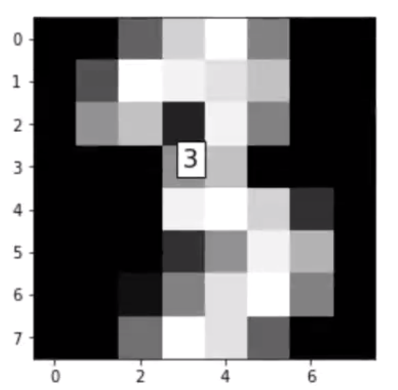
I believe this digit is: 9
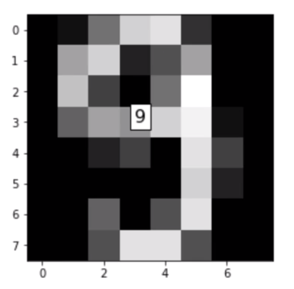
If we are already satisfied with the result of the model, we can use it to meet the ultimate purpose of making new predictions.

KNN Classification in Python — Predictions on New Data with the Trained Model

After we train the model and evaluate its performance, we can use the model to make predictions with new data — in this case; it is intended to make digit predictions.

Below is a list that represents the pixels of a digit from 0 to 10. We have the 64 variables where each position is a pixel of any digit — the digit is an image in a two-dimensional matrix converted into a vector.

# Setting a new digit (input data)
newDigit = [0., 0., 0., 8., 15., 1., 0., 0., 0., 0., 0., 12., 14., 0., 0., 0., 0., 0., 3., 16., 7., 0., 0., 0., 0., 0., 6., 16., 2., 0., 0., 0., 0., 0., 7., 16., 16., 13., 5., 0., 0., 0., 15., 16., 9., 9., 14., 0., 0., 0., 3., 14., 9., 2., 16., 2., 0., 0., 0., 7., 15., 16., 11., 0.]

Next, we need to normalize the data since the model learned from normalized data.

# Normalizing the new digit
newDigit_norm = newDigit - X_norm

We pass the normalized digit as a parameter for finalModel prediction:

# Making the prediction with the trained model
newPrediction = finalModel.predict([newDigit_norm])

Below we take the pixels, put them back in a two-dimensional matrix format, adjust the scale, and print:

# Model prediction
imgdata = np.array(newDigit, dtype='float')
pixels = imgdata.reshape((8,8))
plt.imshow(pixels, cmap='gray')
plt.annotate(newPrediction,(3,3), bbox={'facecolor':'white'},fontsize=16)
print("I believe this digit is: {}".format(newPrediction))
plt.show()
I believe this digit is: [6]
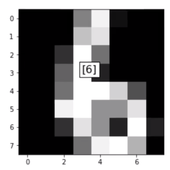
And there we have it. Our model is working. With this, we complete the KNN model for digit predictions. I hope you have found this helpful. Thank you for reading. ?


K-nearest neighbors algorithm detailed in Python was originally published in Level Up Coding on Medium, where people are continuing the conversation by highlighting and responding to this story.


This content originally appeared on Level Up Coding - Medium and was authored by Anello


Print Share Comment Cite Upload Translate Updates
APA

Anello | Sciencx (2021-06-09T02:27:52+00:00) K-nearest neighbors algorithm detailed in Python. Retrieved from https://www.scien.cx/2021/06/09/k-nearest-neighbors-algorithm-detailed-in-python/

MLA
" » K-nearest neighbors algorithm detailed in Python." Anello | Sciencx - Wednesday June 9, 2021, https://www.scien.cx/2021/06/09/k-nearest-neighbors-algorithm-detailed-in-python/
HARVARD
Anello | Sciencx Wednesday June 9, 2021 » K-nearest neighbors algorithm detailed in Python., viewed ,<https://www.scien.cx/2021/06/09/k-nearest-neighbors-algorithm-detailed-in-python/>
VANCOUVER
Anello | Sciencx - » K-nearest neighbors algorithm detailed in Python. [Internet]. [Accessed ]. Available from: https://www.scien.cx/2021/06/09/k-nearest-neighbors-algorithm-detailed-in-python/
CHICAGO
" » K-nearest neighbors algorithm detailed in Python." Anello | Sciencx - Accessed . https://www.scien.cx/2021/06/09/k-nearest-neighbors-algorithm-detailed-in-python/
IEEE
" » K-nearest neighbors algorithm detailed in Python." Anello | Sciencx [Online]. Available: https://www.scien.cx/2021/06/09/k-nearest-neighbors-algorithm-detailed-in-python/. [Accessed: ]
rf:citation
» K-nearest neighbors algorithm detailed in Python | Anello | Sciencx | https://www.scien.cx/2021/06/09/k-nearest-neighbors-algorithm-detailed-in-python/ |

Please log in to upload a file.


There are no updates yet.
Click the Upload button above to add an update.

You must be logged in to translate posts. Please log in or register.