This content originally appeared on HackerNoon and was authored by Kinetograph: The Video Editing Technology Publication
:::info Authors:
(1) Joshua P. Ebenezer, Student Member, IEEE, Laboratory for Image and Video Engineering, The University of Texas at Austin, Austin, TX, 78712, USA, contributed equally to this work (e-mail: joshuaebenezer@utexas.edu);
(2) Zaixi Shang, Student Member, IEEE, Laboratory for Image and Video Engineering, The University of Texas at Austin, Austin, TX, 78712, USA, contributed equally to this work;
(3) Yixu Chen, Amazon Prime Video;
(4) Yongjun Wu, Amazon Prime Video;
(5) Hai Wei, Amazon Prime Video;
(6)Sriram Sethuraman, Amazon Prime Video;
(7) Alan C. Bovik, Fellow, IEEE, Laboratory for Image and Video Engineering, The University of Texas at Austin, Austin, TX, 78712, USA.
:::
Table of Links
- Abstract and Introduction
- Related Work
- Details of Subjective Study
- Subjective Analysis
- Objective Assessment
- Conclusion, Acknowledgment and References
V. OBJECTIVE ASSESSMENT
A. Full Reference Video Quality Assessment
We tested the Peak Signal to Noise Ratio (PSNR), the Structural Similarity Index Measure (SSIM) [13], Multi-Scale SSIM (MS-SSIM) [31], Video Multimethod Assessment Fusion (VMAF) [14], Spatio-Temporal Reduced Reference Entropic Differences (STRRED) [16], Spatial Efficient Entropic Differencing (SpEED) [15], and the Space-Time GeneRalized Entropic Difference (STGREED) [17] video quality models on the newly created database. We evaluated the FR VQA algorithms by computing the Spearman’s Rank Ordered Correlation Coefficient (SRCC) between the scores predicted by the algorithms and the ground truth DMOS. We also fit the predicted scores to the DMOS using a logistic function
\

\

\

\

\ and then computed Pearson’s Linear Correlation Coefficient (LCC) and the Root Mean Square Error (RMSE) between the fitted scores and the DMOS, following standard practice [32]. The results are presented in Table II .
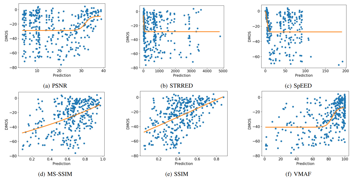
\ As can be seen, the FR metrics did not perform well on the task, with VMAF achieving the highest SRCC of 0.56 on TV1, 0.55 on TV2, and 0.59 on TV3. In addition, since none of these models incorporate modelling of the display device, their predictions were the same on all three televisions, except for STGREED which requires an SVR to be trained separately for each TV. These results underscore the need for further research on FR VQA for HDR and SDR content. The predictions are plotted against the scores obtained for TV1 in Fig.7.
\ B. HDRPatchMAX
Motivated by the low performance of existing models, we also designed a new HDR NR-VQA algorithm called HDR PatchMAX. HDRPatchMAX utilizes features that are relevant to SDR and HDR quality, as well as to motion perception.
\ 1) NIQE features: The first set of features in HDRPatchMAX are the same as those in NIQE [24]. NIQE can be used alone as a blind metric, but we average the 36 features and the distance measure across all frames in each video and use the resulting 37 features for subsequent training.
\ 2) PatchMAX: The 37 features obtained from NIQE performed strongly on the LIVE HDR, LIVE AQ HDR, and LIVE HDRvsSDR dataset, which prompted us to develop a patch-based feature extraction method. We start by partitioning the frame into non-overlapping patches of size P × P and computing their Mean Subtracted Contrast Normalization (MSCN) coefficients. The MSCN coefficients Vˆ [i, j, k0] of a luma channel of a video frame or patch V [i, j, k0] are defined as :
\

\ where i ∈ 1, 2.., M, j = 1, 2.., N are spatial indices, M and N are the patch height and width, respectively, the constant
\

\

\ TABLE II: Median SRCC, LCC, and RMSE of FR VQA algorithms on the new LIVE HDRvsSDR Database. Standard deviations are in parentheses. Best results for each TV are in bold.
\

\ C imparts numerical stability, and where
\
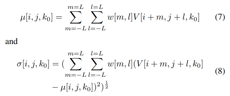
\ are the local weighted spatial mean and standard deviation of luma, respectively. The weights w = {w[m, l]|m = −L, . . . , L, l = −L, . . . , L} are a 2D circularly-symmetric Gaussian weighting function sampled out to 3 standard deviations and rescaled to unit volume, and K = L = 3.
\ The standard deviation that is computed during the MSCN operation is averaged across each patch and is used as a proxy for each patch’s contrast. The patches are then divided into three groups based on the percentile of their standard deviation relative to the standard deviation of the other patches in the frame. High contrast patches are defined as patches having standard deviations above the (100 − T) th percentile, medium contrast patches are defined as patches with standard deviations between the T th and (100 − T) th percentiles, and low contrast patches are those having standard deviations less than the T th percentile.
\ The MSCN coefficients of these patches can be reliably modelled as Generalized Gaussian Distributions (GGD), defined as
\

\ where Γ(.) is the gamma function:
\

\ The shape and variance parameters of the best fit to the MSCN coefficients, α and β, are extracted and used as quality-aware features.
\ Following this, compute the products of neighboring pairs of pixels in each patch to capture correlations between them
\
\ as follows:
\

\ These are modelled as following an Asymmetric Generalized Gaussian Distribution (AGGD):
\

\ where
\

\ and where ν controls the shape of the distribution and σl and σr control the spread on each side of the mode. The parameters (η, ν, σ2 l , σ2 r ) are extracted from the best AGGD fit to the histograms of each of the pairwise products in (11), where
\

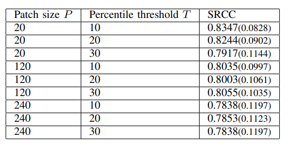
\ The parameters of the best fit to each patch are extracted as quality features, and are averaged separately for each of the three categories of patches, yielding a total of 54 features. This procedure is performed at two scales to yield a total of 108 features. In addition to this, we also compute the average temporal standard deviation of these features over every nonoverlapping group of five consecutive frames, and use the additional 108 features as spatio-temporal quality features. The patch size P and the percentile threshold T are treated as hyperparameters, and were chosen as P = 20 and T = 10 based on the results shown in Table III.
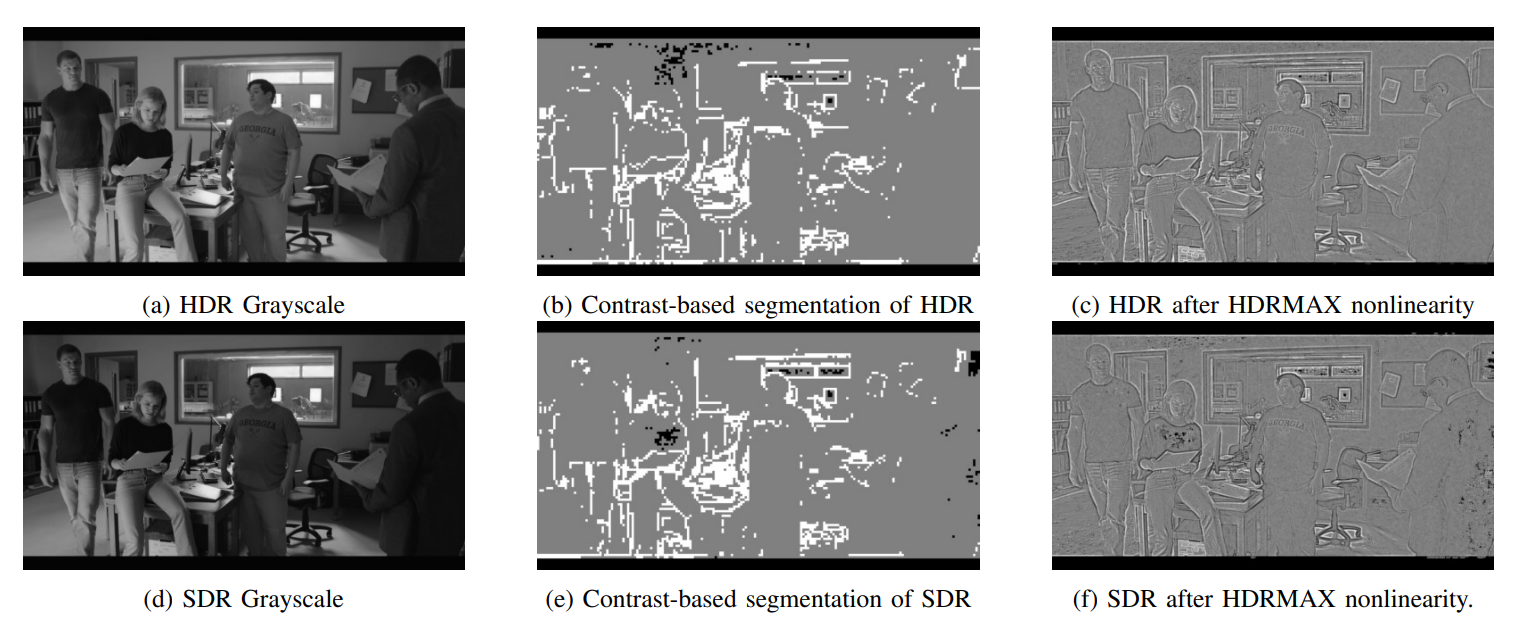
\ There are three important motivations for the use of contrast-separated feature aggregation. Firstly, one of the primary ways HDR differs from SDR is in its representation of local contrast. SDR frames, being limited to 8 bits, cannot represent edges and details as well as HDR frames are. However, feature responses corresponding to this increased contrast visibility may be masked by feature responses from other regions of the frame which may not benefit from the more accurate quantization of HDR. Explicitly separating feature responses by contrast prevents this masking effect. For example, in Fig. 8(b), high contrast regions of an HDR frame are shown in white, medium contrast regions are shown in gray, and low contrast regions are shown in black. In Fig. 8(e), the same is shown for the SDR version of the same frame. In the SDR version, there are underexposed regions in the woman’s t-shirt and in the back of the suit worn by the man in the foreground, which are highlighted as low-contrast regions by our proposed contrast-based segmentation. In the HDR version, the same regions are not underexposed and lowcontrast regions are instead only located in the plain walls in the background. The statistics of these regions will accordingly be different and quality-aware.
\ Secondly, NSS modelling suffers in the presence of regions of very low contrast (such as the sky). Prior observations on the Gaussianity of MSCN coefficients of pristine frames are strongly validated by most natural scenes, very smooth areas lacking any texture or detail can present rare exceptions to this natural law. Separating such areas from regions of higher contrast and texture may therefore improve the validity and power of these models.
\ Thirdly, contrast masking is an important visual phenomenon whereby distortions may become less visible in the presence of high contrast textures, providing additional motivation for separately analyzing regions having different contrasts. The MSCN operation serves to model the contrastgain masking that occurs in the early stages of the human visual system, while the explicit separation of regions with different contrasts contributes to additional modelling of this effect.
\ The MSCN coefficients of different patches grouped by their contrasts are plotted in Fig. 9 for a frame from a compressed HDR video, along with the corresponding SDR frame. The coefficients clearly differ and the best GGD fits to these distributions will be accordingly quality-aware.
\ 3) HDRMAX: The HDRMAX feature set [33] is extracted by first passing the luma values of each frame through an expansive nonlinearity, first introduced in HDR ChipQA. Values in overlapping windows of size 20 × 20 are first linearly rescaled to [−1, 1] using the minimum and maximum values in each window. They are then passed through an expansive nonlinearity defined as follows:
\

\ where δ = 4 based on prior experiments [33] on the LIVE HDR database. This nonlinearity amplifies local contrasts by suppressing the middle range of values and by amplifying the extreme ends of the luminance range. Since HDR excels in representing contrasts, this operation enhances endemic compression distortions and forces subsequent feature responses to focus on them
\ In Fig. 8(c) and Fig. 8(f), for example, the HDRMAX nonlinearity is applied to the frames shown in Fig. 8(a) and Fig. 8(d), respectively. Local contrast is amplified in the resulting images throughout the frame. Regions in SDR suffering from underexposure, such as the woman’s t-shirt, and overexposure, such as the tubelight in the room behind, present luminance values that are near constant and are hence stretched to extremes with sharp boundaries that highlight their defects. The corresponding regions in the HDR version are smoother, and distortions in those regions highlight HDR’s enhanced ability to represent contrast.
\ The MSCN coefficients of the nonlinearly processed frames are computed and modelled as following a GGD, and their neighboring products are modelled as following an AGGD, yielding 18 features. These features are extracted at two scales. In addition, we also find the average standard deviation of these features on every non-overlapping group of five frames, yielding 72 features.
\ 4) Space-Time Chips: We model spatio-temporal information using Space-Time (ST) Gradient Chips, first introduced in [34] and further developed in [22]. Gradients carry important information about edges and distortions and ST chips are spatiotemporal slices of the gradient video that are designed to capture temporal information in a quality-aware way. The
\ TABLE III: Effect of varying patch size and percentile thresholds on median SRCC for TV1.
\
\ gradient magnitude of each frame is first computed using a 3 × 3 Sobel operator. The MSCN coefficients of the gradient magnitude are found using Eqn. (6). Following this, a temporal bandpass filter k(t) is applied:
\

\ This simple linear filter models the process of temporal decorrelation that occurrs in the lateral geniculate nucleus (LGN) [35]. The visual signal passes to area V1 from the LGN, where neurons are sensitive to motion over local areas. Motivated by this, spatiotemporal slices of the MSCN coefficients of the gradient video are selected from each spatial location by performing a grid search over six directions, and by selecting the slice having the kurtosis closest to that of a Gaussian.
\ Specifically, let Gˆ[i, j, k] denote MSCN coefficients of the gradient magnitudes of video frames with temporal index k. For k = T, define a block of 5 frames ending at time T, denoted Gˆ T = Gˆ[i, j, k]; k = T − 4, . . . T. Then, within each space-time volume Gˆ T , define six 5x5 space-time slices or chips, which intersect all 5 frames, which are separated by an angle of π 6 , and are constrained so that the center of each chip coincides with the center of the volume Gˆ T , and so that the normal vector of every chip lies on the spatial plane. ST chips that are perpendicular to the direction of motion will capture the motions of objects along that vector, where we tacitly assume that motions of small spatiotemporal volumes is translational. We have previously shown that the natural bandpass statistics of ST chips of high-quality videos that are oriented perpendicular to the local direction of motion reliably follow a Gaussian law, while those pointing in other directions diverge from Gaussianity [22]. This observation follows from the Gaussianity of MSCN coefficients of pristine frames. Accordingly, in each 5 × 5 × 5 volume, we select the 5 × 5 ST chip that has the least excess kurtosis. The ST Gradient chips coefficients are modelled as following a GGD, and their neighboring pairwise products are modelled as following an AGGD, yielding 18 features. This procedure is repeated at two scales, yielding a total of 36 features.
\ HDRPatchMAX hence consists of 37 NIQE features, 108 PatchMAX features, 72 HDRMAX features, and 36 ST Gradient Chip features.
\
\

\ C. No-Reference Video Quality Assessment
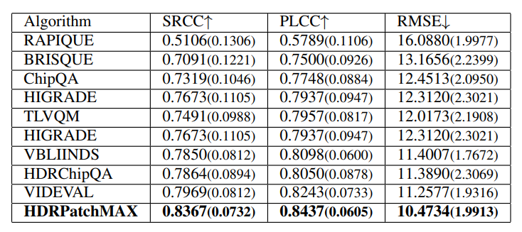
We evaluated RAPIQUE [21], BRISQUE [18], TLVQ [25], VBLIINDS [19], ChipQA [22], and HDR ChipQA [23], as well as HDRPatchMAX, on the new LIVE HDRvsSDR Database. Again, we report the SRCC, PLCC, and RMSE metrics. The algorithms were trained using a Random Forest Regressor. We also tested the Support Vector Regressor but chose the Random Forest Regressor based on its better performance. The videos are separated into training and test sets with an 80:20 ratio such that videos of the same content appeared in the same set. Cross-validation was performed over the training set to select the best hyperparameters (the number of estimators and the number of features) for the random forest. The random forest with the best hyperparameters was then fitted to the training set and evaluated on the test set. This procedure was repeated 100 times with different randomized train-test splits, with the median results reported along with the standard deviations in Table IV. HDRPatchMAX outperformed the other NR VQA algorithms on all the televisions. The parameters P and T were chosen based on the performance of the PatchMAX set of features as P and T were varied, as reported in Table III.
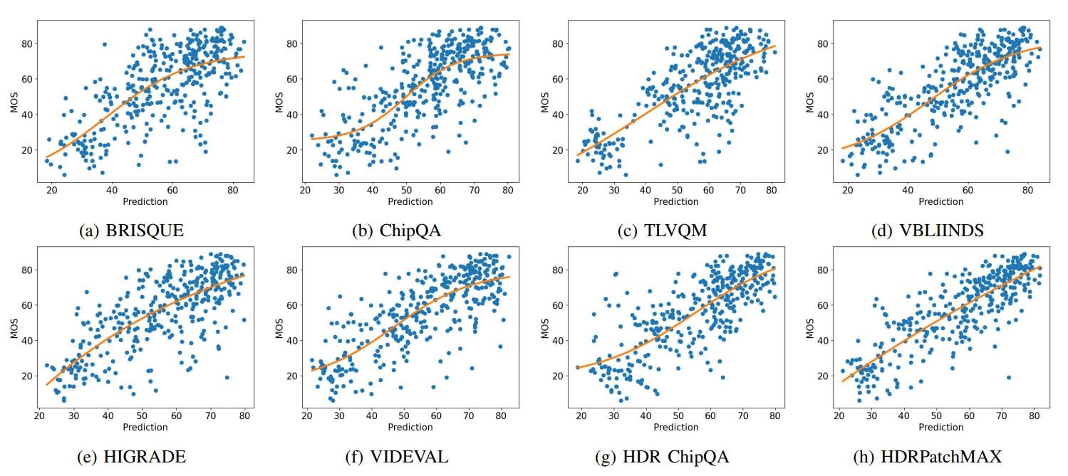
\ The scatter plots of the predictions made by the NR VQA algorithms against the MOS obtained on the videos shown on TV1 are shown in Fig. 10. The scatter plots were created by plotting the MOS against the mean quality predictions produced by the NR VQA algorithms on each video in the test set over the 100 train-test splits, using the logistic fit in Eqn. 5 shown in orange. HDRPatchMAX’s predictions are better aligned with MOS and have a more linear fit than the other algorithms.
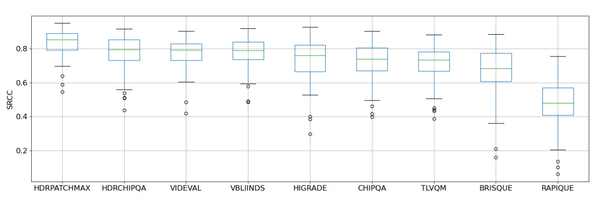
\ We also show a boxplot of the SRCCs obtained over the 100 train-test splits by the NR VQA algorithms on TV1 in Fig. 11. HDRPatchMAX has a higher median SRCC and a tighter spread of values than the other algorithms.
\ We also evaluated each feature set in HDRPatchMAX individually, and report the results in Table V for TV1. The PatchMAX set of features obtained the highest performance and individually exceeded the performance of other NR VQA algorithms. We also conducted an ablation study with HDRPatchMAX, removing each feature set and evaluating the performance of the rest of the feature sets on TV1, and report the results in Tab. VI. Despite the strong individual performance of PatchMAX, its removal had minimal impact on the algorithm’s performance, indicating the robustness and complementary nature of the other feature sets. Similar results were observed on TV2 and TV3.
\ TABLE IV: Median SRCC, LCC, and RMSE of NR VQA algorithms on LIVE HDRvsSDR. Standard deviations are in parentheses. Best results for each TV are in bold.
\

\
\
\ TABLE V: Individual feature performance on TV1.
\

\ TABLE VI: Ablation study on TV1.

\ The random forest models trained on the data from TV1, TV2, and TV3, can be considered as separate models for OLED displays, QLED displays, and LED displays respectively. However, we also conducted a separate experiment where each TV was assigned a numerical value (1 for TV1, 2 for TV2, and 3 for TV3) that was concatenated onto each NR VQA algorithm as an additional feature, and trained on the scores obtained from all the display devices, treating videos shown on different display devices as different stimuli with different feature vectors. The results are shown in Table VII. HDRPatchMAX once again is the leading performer.
\ D. Results on combined databases
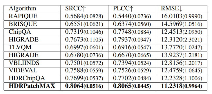
We evaluated the NR and FR VQA algorithms on the combined LIVE HDR, LIVE AQ HDR, and LIVE HDRvsSDR databases consisting of 891 HDR videos and 175 SDR videos. The Samsung Q90T (TV2) was used for the LIVE HDR and LIVE AQ HDR studies, so the scores from the LIVE HDR and LIVE AQ HDR databases were mapped to the scores obtained from from TV2 in the LIVE HDRvsSDR database using the procedure described in Section IV-D, and then used as the ground truth for evaluation. The results are presented in Table VIII for FR metrics and Table IX for NR metrics. HDRPatchMAX was the best performer on the combined dataset among NR VQA models while VMAF was the best performer among FR VQA models.
\ TABLE VII: Results on all display devices using TV indices as additional features.
\
\ TABLE VIII: Median SRCC, LCC, and RMSE of FR VQA algorithms on the combined databases. Standard deviations are in parentheses. Best results are in bold.
\

\ TABLE IX: Median SRCC, LCC, and RMSE of FR VQA algorithms on the combined databases. Standard deviations are in parentheses. Best results are in bold.
\
\
:::info This paper is available on arxiv under CC 4.0 license.
:::
\
This content originally appeared on HackerNoon and was authored by Kinetograph: The Video Editing Technology Publication
Kinetograph: The Video Editing Technology Publication | Sciencx (2024-07-08T12:00:20+00:00) HDR or SDR? A Study of Scaled and Compressed Videos: Objective Assessment. Retrieved from https://www.scien.cx/2024/07/08/hdr-or-sdr-a-study-of-scaled-and-compressed-videos-objective-assessment/
Please log in to upload a file.
There are no updates yet.
Click the Upload button above to add an update.
