This content originally appeared on Level Up Coding - Medium and was authored by Shitanshu Bhushan

Continuing in our series of from-scratch implementations, we will implement the famous ResNet-50 architecture using pytorch in this article! Deviating from my previous articles, we will first see the code and then break it down to understand the most important concepts for any neural network.
Architecture of ResNet
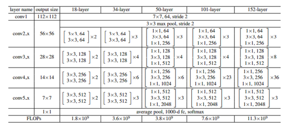
Back in the early 2010s, ever since AlexNet won the 2012 ImageNet competition, there was this push to make these architectures deeper which just means to add more and more layers but researchers found that just increasing the depth did not lead to performance gains, instead the deeper models were actually performing worse than their shallow counterparts. The reason for this was found to be vanishing/exploding gradients. So in 2015, researchers from Microsoft introduced residual network architecture, where they use shortcut/skip connections to allow the gradients to flow more easily through the network.
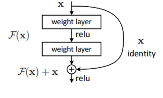
Regarding ResNet-50, researchers introduced these bottleneck architectures where we first reduce the dimension using a 1x1 convolution, then perform the main computation with a 3x3 convolution, and finally restore the dimensionality with another 1x1 convolution. The main goal of this bottleneck is to reduce computation and increase efficiency due to constraints on training time.
ResNet-50 from scratch implementation
Okay let’s see what this architecture looks like in code,
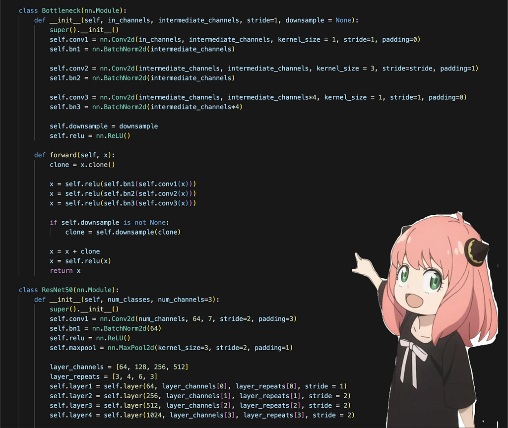
The above code is based on: pytorch resnet code
It will be quite difficult to explain the code in one go, so I will break it down into smaller chunks to explain the architecture step by step, but first let’s understand some common topics:
Convolutions
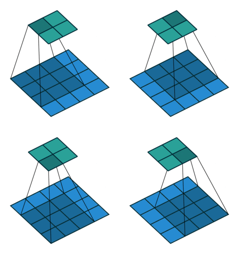
In the architecture we saw stuff like 1x1 convolution or 7x7 convolution but what exactly does that mean? Convolutions can simply be thought of as sliding a filter over the entire input, the filter at each position then performs element-wise multiplication and summation producing feature maps that capture local information like edges, etc. and it’s these filter weights that we then end up learning during training! A key point to remember is that these filters always extend the full depth of the input volume. Convolutions are usually preferred over fully connected layers for images as they capture local data much better by preserving spatial relationships between pixels and also reduce the total number of parameters to be learned.
Some key terms to remember here are:
- Strides — This is used to specify the step size by which the filter moves across the input
- Padding — This is used to specify the addition of extra pixels in the input to control the dimension of the output and preserve border information.
- Kernel size — This is the size of our filter described as height x width
- In channels — This is the number of input channels
- Out channels — This is the number of output channels produced by the convolution layer
A key formula to remember for convolutions is:

The above formula is quite useful to determine what the padding or stride should be when not explicitly told.
Why do we need Batch Normalization?
Batch Normalization is a widely adopted technique that enables faster and more stable training of deep neural networks. Batch normalization standardizes the inputs of each layer to have a mean of 0 and a variance of 1 within each mini-batch. When it was first introduced in 2015, the reason for this faster and more stable training was said to be that batch normalization reduces internal covariance shift but in a 2019 paper the authors argued that BatchNorm impacts network training by making the loss landscape significantly smoother and that in turn helps in training a network.
Why do we need Non-linearity?
We introduce nonlinearity(ReLU) in our architecture so that we can learn complex, non-linear decision boundaries. If we didn’t use the non-linearities then our model would just be a stack of linear operations regardless of its depth.
Why do we need Pooling?
Pooling reduces the spatial dimension of the feature maps, which helps reduce the computational load and number of parameters. It operates over each activation map independently. Pooling helps in extracting sharp (maxpool) and smooth (avgpool) features. The work of pooling could also be done by convolution by increasing the stride but pooling is faster to compute than convolutions.
Code Walkthrough
Okay now let’s go over the code to understand what each part is doing

Okay so first our input is of shape [batch size, channels, height, width], which for us is [1, 3, 224, 224]. It first passes through a 7x7 convolution with stride 2 and padding 3, then through batch normalization and then a ReLU. It then passes through a 3x3 maxpool with stride 2 and padding 1 to have a final dimension of [1, 64, 56, 56]. A good way to test whether your architecture is given the right dimension or not is to pass a random tensor to see what the shape of the output is.
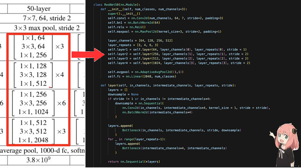
Okay, next we will focus on these layers. In each layer, the output channels are 4*intermediate channels, and each layer is made up of the bottleneck blocks repeated a certain amount of times. The layer_channels array holds the intermediate channels for that layer of the bottleneck, layer_repeats array holds the number of times each layer is repeated. For each layer we call a function “layer” which returns a sequential container of the order of each operation in that layer. Each layer is made up of bottleneck blocks which we will see next
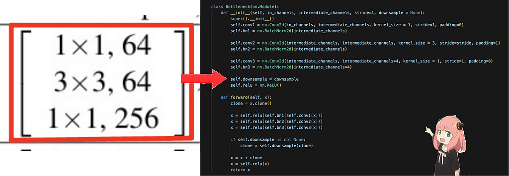
In each bottleneck block, the convolutions are applied in the order as described above, and at the end, we add the input back into the output for the residual connection. The downsample part is required to make sure the input is converted to the same spatial dimension as the output so that they can be added together.
After all these layers, we finally do an adaptive average pool and then pass it through a fully connected layer with the desired number of output classes to get the final output.
I tested my implementation on CIFAR-10, my from-scratch implementation after 10 epochs of training got an accuracy of 75%, and training resnet50 from pytorch with pretrained=False got an accuracy of 77%.
Summary
As we saw above, pretty simple to implement ResNet on your own and it’s a very good model to implement to learn the basics from. ResNet’s use of residual connections simplifies the training of deep networks and offers a great way to understand the challenges and solutions associated with deep learning architectures. In terms of application, CNNs in general are extremely popular in the field of computer vision for tasks like image classification, object detection, segmentation, etc.
All the code for this can be found at — ResNet from scratch
Deeper is better: Coding ResNet from scratch was originally published in Level Up Coding on Medium, where people are continuing the conversation by highlighting and responding to this story.
This content originally appeared on Level Up Coding - Medium and was authored by Shitanshu Bhushan
Shitanshu Bhushan | Sciencx (2024-07-25T00:24:22+00:00) Deeper is better: Coding ResNet from scratch. Retrieved from https://www.scien.cx/2024/07/25/deeper-is-better-coding-resnet-from-scratch/
Please log in to upload a file.
There are no updates yet.
Click the Upload button above to add an update.
