
This content originally appeared on HackerNoon and was authored by Economic Hedging Technology
Table of Links
1.2 Asymptotic Notation (Big O)
1.5 Monte Carlo Simulation and Variance Reduction Techniques
- Literature Review
- Methodology
3.2 Theorems and Model Discussion
4. RESULT ANALYSIS
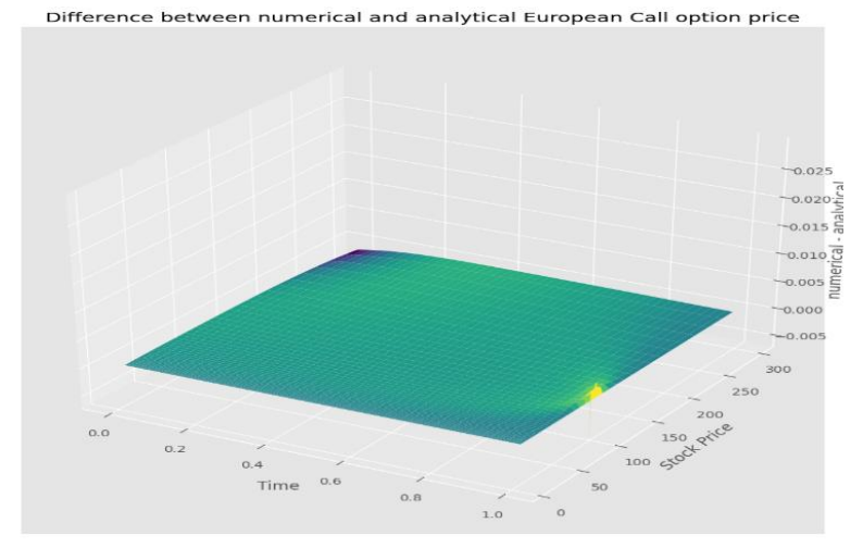
We use the parameters listed in (3) to generate data for options to verify our results from the European call option against the analytical solution given in (3) in order to confirm their accuracy. This comparative analysis provides a thorough assessment of the efficacy of the data we generate in comparison to the existing solution. When comparing the results of predicting call options by the finite difference method (FDM) and analytically, there are many things to take into account. Both these ways try to approximate the price of a call option but with different methods. So, let me consider these two methods in detail:
\ Finite Difference Method (FDM):
\ The partial differential equation that governs the pricing of options is discretized in a grid by FDM and solved numerically [31]. The sizing of the grid, as well as whether to use explicit, implicit, or Crank-Nicolson numerical schemes, are among the factors that affect its accuracy. Making sure that FDM solutions converge is very important. This may not happen if a grid is used too coarsely or when an unstable numerical scheme is adopted, thereby leading to wrong answers. FDM can consume a lot of computer resources particularly with difficult option structures or problems having many dimensions. Time complexity grows as grid size increases together with the number time steps required for convergence. This allows early exercise features to be included as well as dividends or changes in volatility over time. Nonetheless, complex functionality implementation within FDM needs carefulness while also increasing computational complexities [32].
\
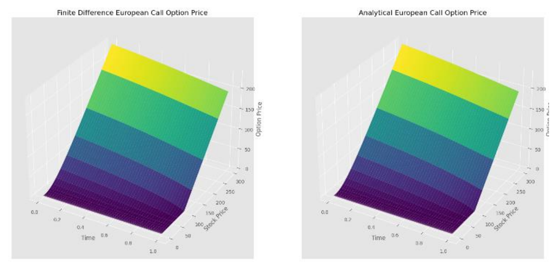
\ The Black-Scholes model is an example of an analytical method that can provide a closed-form solution for pricing options given certain assumptions (for instance, constant volatilities with no dividends). This type of solution tends to be simpler and faster computationally than numerical ones like FDM. It is important to note that all analytic methods make some assumptions which may not hold true in reality. One such assumption made by the Black-Scholes model is that the volatility remains constant and the risk-free rate is continuously compounded. If any of these conditions are violated, then there will be disparities between what the market price says should happen according to this formula versus how things actually turn out.
\ Comparative Analysis:
\ FDM gives greater precision and accuracy, particularly for involved option structures or payoffs that aren't linear. However, the added computational complexity and resource utilization required to achieve this level of precision make it expensive.
\
\ Computational efficiency is what analytical methods are all about; they prioritize simplicity over anything else. They may lose some of their precision when assumptions within models do not hold true which doesn’t always happen often except for in unique cases. FDM is a more robust method than its counterpart analytic because it can deal with different types of options under various market situations. This means that FDM can handle changes in parameters and boundary conditions as they occur when compared against dynamic treatment using an equation solver like the Runge-Kutta method. Analytical techniques lack this flexibility while being efficient at processing large amounts of data quickly but need calibration steps where deviations from model assumptions occur, thereby limiting them to only ideal scenarios during testing stages before real-life applications are used. The choice between FDM and analytic methods is often driven by problem specificity, computational capacity availability, or even trade-offs between accuracy & speed depending on user needs.
\ Monte Carlo Technique:
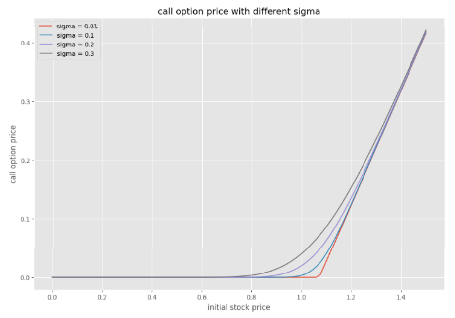
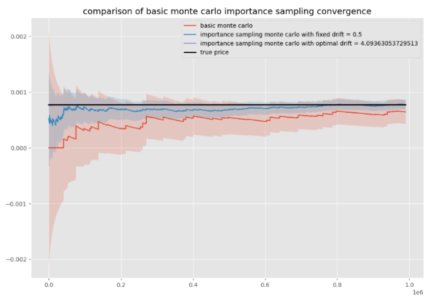
\ Now, we describe some experimental results based on the Monte Carlo method. The fundamental Monte Carlo technique will be covered first, then move on to more advanced methods. In the plot below, take note of the Saw tooth pattern. This is as a result of our raising the option's strike price from 100 to 200. This implies that many fewer simulations result in a profit, leading to extended periods during which the Monte Carlo price falls; conversely, when the option is profitable, the Monte Carlo price rises significantly [33].
\
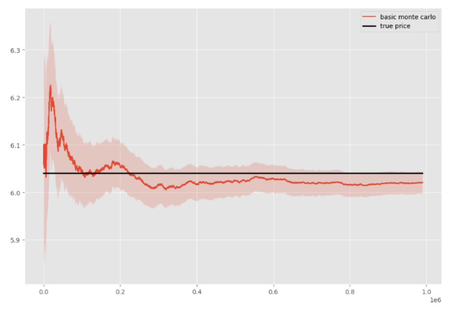
\ The fundamental concept is to compute the payoff of the derivative after simulating the price of the underlying asset at the derivative's maturity. The average of the payoffs discounted to the present is the derivative's price [34]. Comparing simulated option prices with those derived from traditional pricing models assesses the efficacy of Monte Carlo simulation in capturing the complexities of market dynamics and volatility. Results highlight the flexibility and adaptability of Monte Carlo simulation in modeling various scenarios, shedding light on its potential as a robust tool for options pricing. The analysis underscores the importance of considering Monte Carlo simulation as a complementary approach to traditional models, offering insights into risk management and investment strategies in dynamic financial markets [35].
\
\ A large variety of derivatives can be priced using the highly general Monte Carlo approach. However, it is also an extremely slow method that uses a lot of processing resources. Thus, in the next section, we will also examine variance reduction strategies that can be applied to accelerate the Monte Carlo approach.
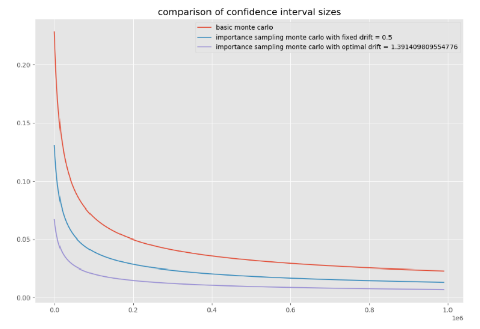
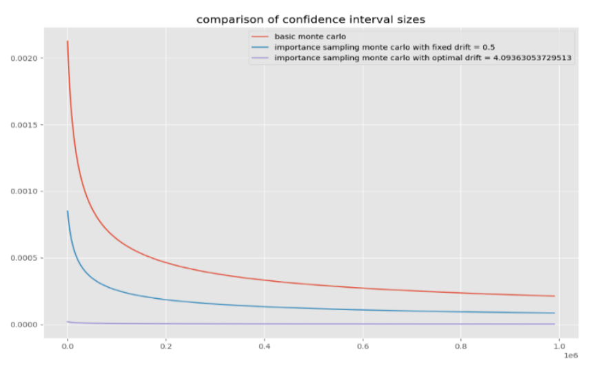
\ Finding a different measure where the estimator's variance is lower is the goal of importance sampling. Reducing variance is the same as reducing the second moment.
\
\
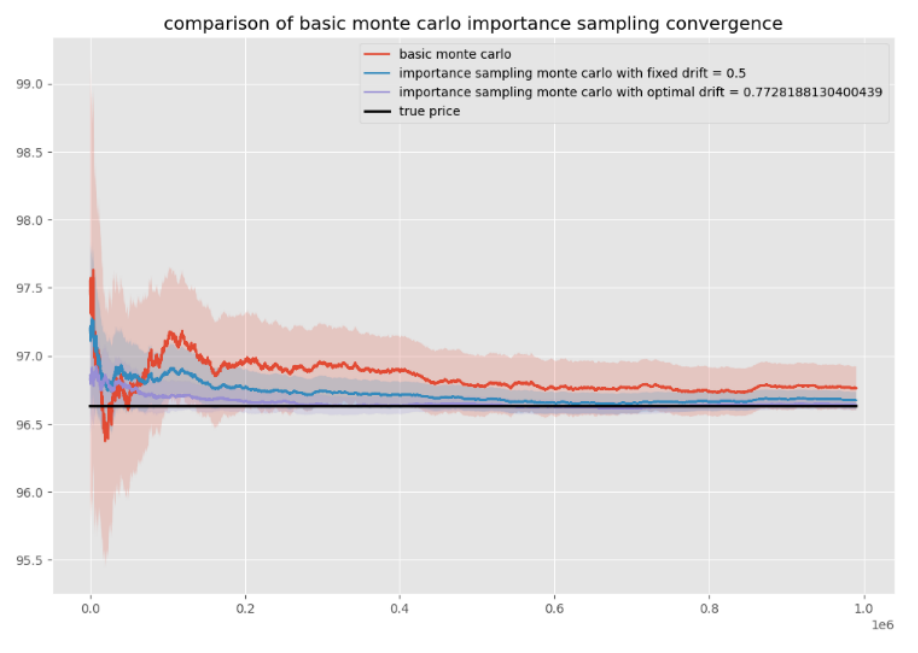
\ Result analysis in Monte Carlo simulation involves assessing the importance of sampling techniques and understanding the significance of confidence intervals. Now, I will increase the strike price value from 100 to 200 and then simulate it again.
\
\
\
\ We can see the changes between Figures (10) and Figure (12), basically in the optimal drift curve. In the second figure, the curve becomes an almost flat line after changing the strike price from 100 to 200.
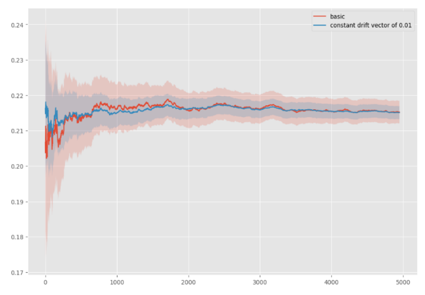
\ We will proceed with importance sampling, but we will now need to sample over several timesteps. As a result, we must deal with a vector of 𝜏 that is made up of random variables. Let's first try a constant 𝜏 for all timesteps.
\
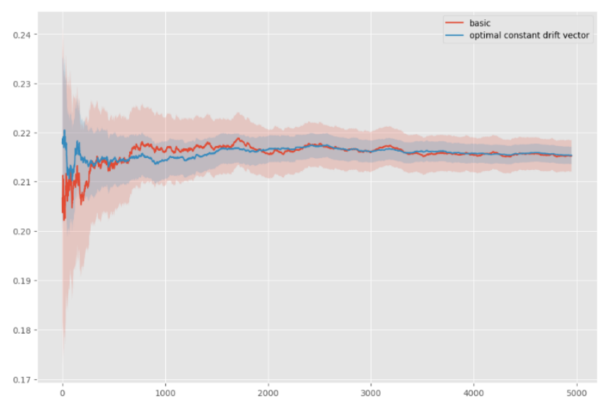
\ Now let's try to find a better 𝜏 for each timestep. We will start by finding the optimal constant 𝜏.
\
\
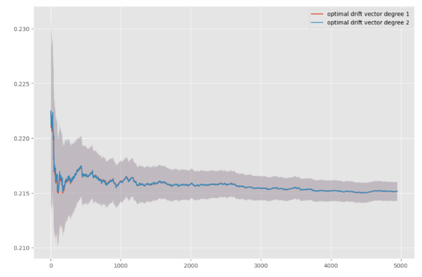
\ After fitting a quadratic function as optimal drift, we can see that there is no difference between degrees 1 and 2. So, it performs well. Let's examine those drift vectors' appearance.
\
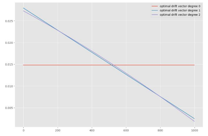
\ Looking closely at how well the optimal drift vector is used in Monte Carlo simulations within the Black-Scholes model can give us some really useful info about how accurate and effective this simulation method is. Assess the convergence properties of Monte Carlo simulations with the optimal drift vector. Evaluate how quickly the simulations converge to stable estimates of option prices or other output metrics.
\ Let's compare in/out of the money and put/call using linear interpolation.
\
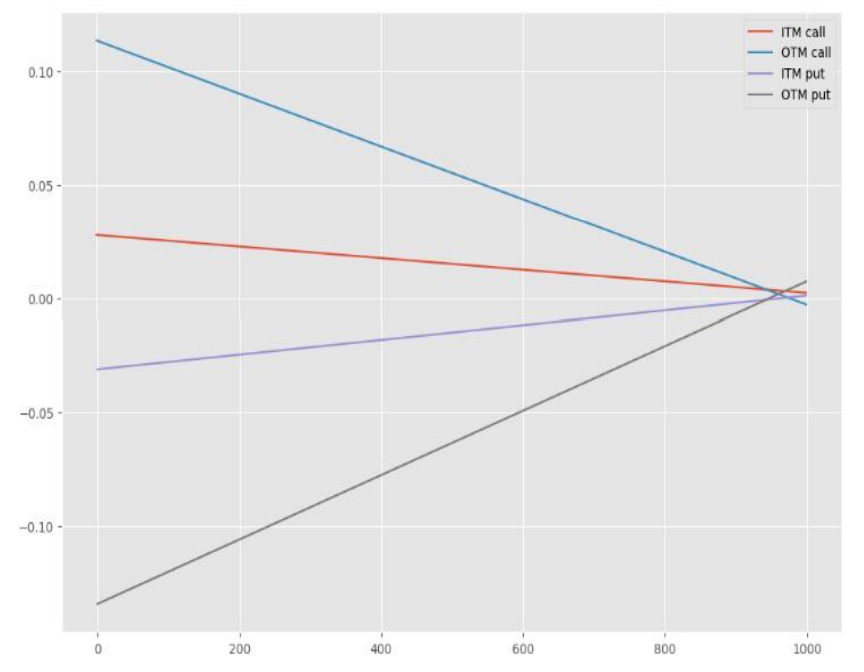
\ We can observe that drift vectors are often decreasing for calls and increasing for puts. This makes basic sense since a reduced variance requires increasing the MC estimator. This indicates that we should add more for out-of-the-money options than for in-the-money options, as well as a negative number for calls and a positive number for puts. By using the Laplace Method, which provides a recursive formula for the ideal 𝜏, this may also be mathematically demonstrated.
\ Antithetic variates exploit negative correlations between pairs of random variables to reduce variance in estimates. In the context of option pricing with the Black-Scholes model, this involves generating two correlated sets of random numbers. The effectiveness of antithetic variates in reducing variance and improving the efficiency of Monte Carlo simulations within the Black-Scholes model can be evaluated through convergence analysis, and comparison with standard Monte Carlo results.
\
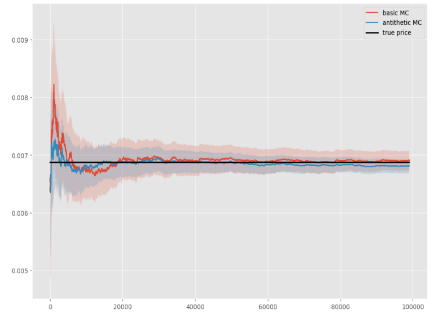
\ This seems very effective for OTM options and is very easy to implement. Note that it is also about twice as expensive computationally as the original method, so for ITM options [36], it is not worth it in this example.
\ Applying control variates in Monte Carlo simulations within the Black-Scholes model can be a powerful technique for reducing the variance of option price estimates, particularly for options that are consistently over or undervalued by the model. Here's how you can apply control variates and analyze the results for in-the-money (ITM) and out-of-the-money (OTM) options:
\
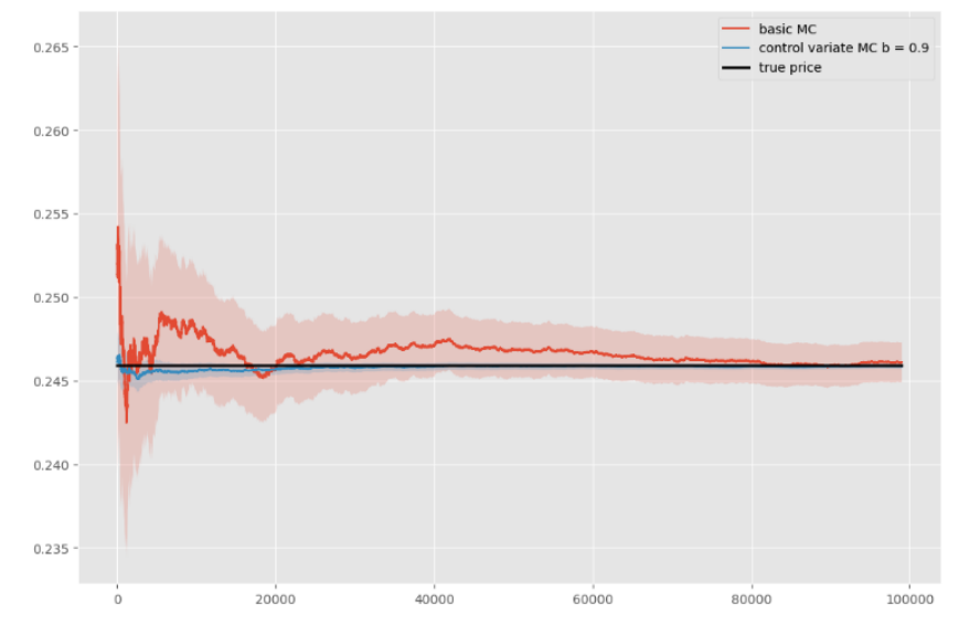
\
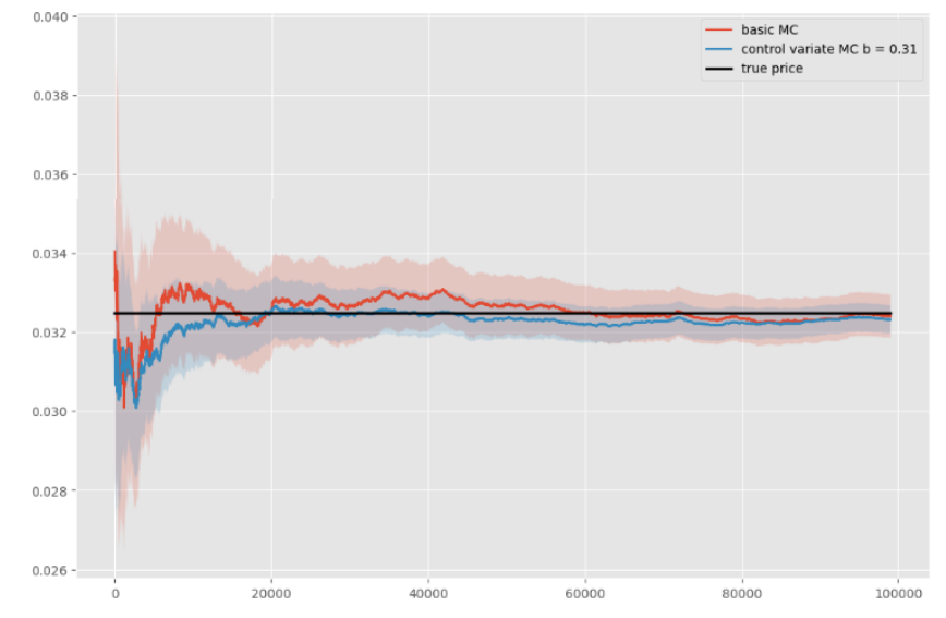
\ For in the money (ITM) we have considered spot price as 1 and the strike price as 0.7, and for the out of the money (OTM) we have considered the strike price as 1.4 with the same spot price and started our experiment after getting the results in terms of the effectiveness of using control variates to improve the accuracy and efficiency of option pricing in the Black-Scholes model.
\
:::info Authors:
(1) Agni Rakshit, Department of Mathematics, National Institute of Technology, Durgapur, Durgapur, India (spiritualagnimath.statml@gmail.com);
(2) Gautam Bandyopadhyay, Department of Management Studies, National Institute of Technology, Durgapur, Durgapur, India (gbandyopadhyay.dms@nitdgp.ac.in);
(3) Tanujit Chakraborty, Department of Science and Engineering & Sorbonne Center for AI, Sorbonne University, Abu Dhabi, United Arab Emirates (tanujit.chakraborty@sorbonne.ae).
:::
:::info This paper is available on arxiv under CC by 4.0 Deed (Attribution 4.0 International) license.
:::
\
This content originally appeared on HackerNoon and was authored by Economic Hedging Technology
Economic Hedging Technology | Sciencx (2024-10-23T06:23:16+00:00) Comparative Analysis of Option Pricing Methods: FDM, Monte Carlo Simulation, and Variance Reduction. Retrieved from https://www.scien.cx/2024/10/23/comparative-analysis-of-option-pricing-methods-fdm-monte-carlo-simulation-and-variance-reduction/
Please log in to upload a file.
There are no updates yet.
Click the Upload button above to add an update.