This content originally appeared on HackerNoon and was authored by Ravi Mandliya
Overview of Large Language Model (LLM) inference, its importance, challenges, and key problem formulations.
\ Large Language Models (LLMs) have revolutionized the field of Natural Language Processing (NLP) by enabling a wide range of applications, from chatbots and AI agents to code and content generation. However, the deployment of LLMs in real-world scenarios often faces challenges related to latency, resource consumption, and scalability.
\ In this series of blog posts, we will explore various optimization techniques for LLM inference. We’ll dive into strategies for reducing latency, memory footprint, and computational cost, from caching mechanisms to hardware accelerations and model quantization.
\ In this post, we will provide a brief overview of LLM inference, its importance, and the challenges associated with it. We will also outline the key problem formulations that will guide our exploration of optimization techniques.
Model Inference: An Overview
Model inference refers to the process of using a trained machine learning model to make predictions or generate outputs based on new input data. In the context of LLMs, inference involves processing text input and generating coherent and contextually relevant text output.
\ Model is trained only once or periodically, while inference occurs far more frequently, probably thousands of times per second in production environments.
\ Inference optimization is essential to ensure that LLMs can be deployed effectively in real-world applications. The goal is to minimize latency (the time taken to generate a response), reduce resource consumption (CPU, GPU, memory), and improve scalability (the ability to handle increasing loads).
\ For example, GPT-3 (with 175 billion parameters) requires significant computational resources for inference. Optimizations can reduce response times from 1–2 seconds to milliseconds, making LLMs more practical for interactive applications.
Overview of Transformer Architecture
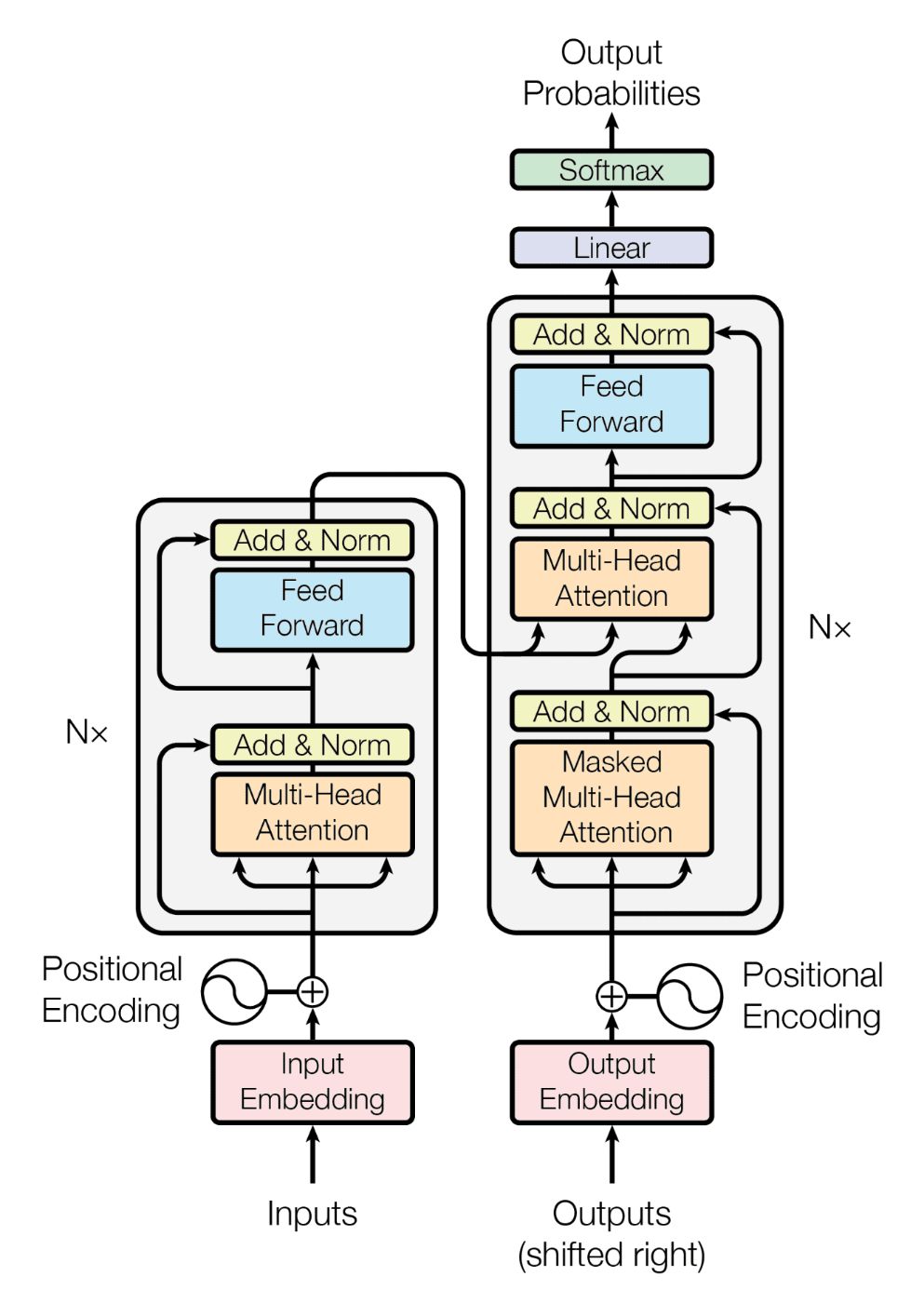
\ The transformer architecture, which uses attention mechanisms, has become the foundation for most state-of-the-art LLMs. This architecture includes positional encodings, multi-head self-attention, feed-forward neural networks, and layer normalization. Transformers are generally classified into three main types:
\
- Encoder-only models (e.g., BERT) are designed for tasks like text classification and named entity recognition. They convert an input sequence into a fixed-length representation - embedding. These models are bi-directional, meaning they consider the context from both the left and right of a token, which can lead to a better understanding of the input text.
\
- Decoder-only models (e.g., GPT-3) are used for text generation tasks. From an input sequence, they generate text one token at a time, conditioning on the previously generated tokens. These models are uni-directional, meaning they only consider the context from the left of a token, which is suitable for tasks like language modeling. This is the most common LLM architecture.
\
Encoder-decoder models (e.g., T5) were the original architecture introduced in the paper “Attention is All You Need.” These models are designed for tasks that require both understanding and generation, such as translation and summarization. They process the input sequence with the encoder and then generate the output sequence with the decoder.
\
Since decoder-only models are the most common LLM architecture for autoregressive tasks, this series will focus on optimization techniques specifically for this type of model.
Overview of the Attention Mechanism
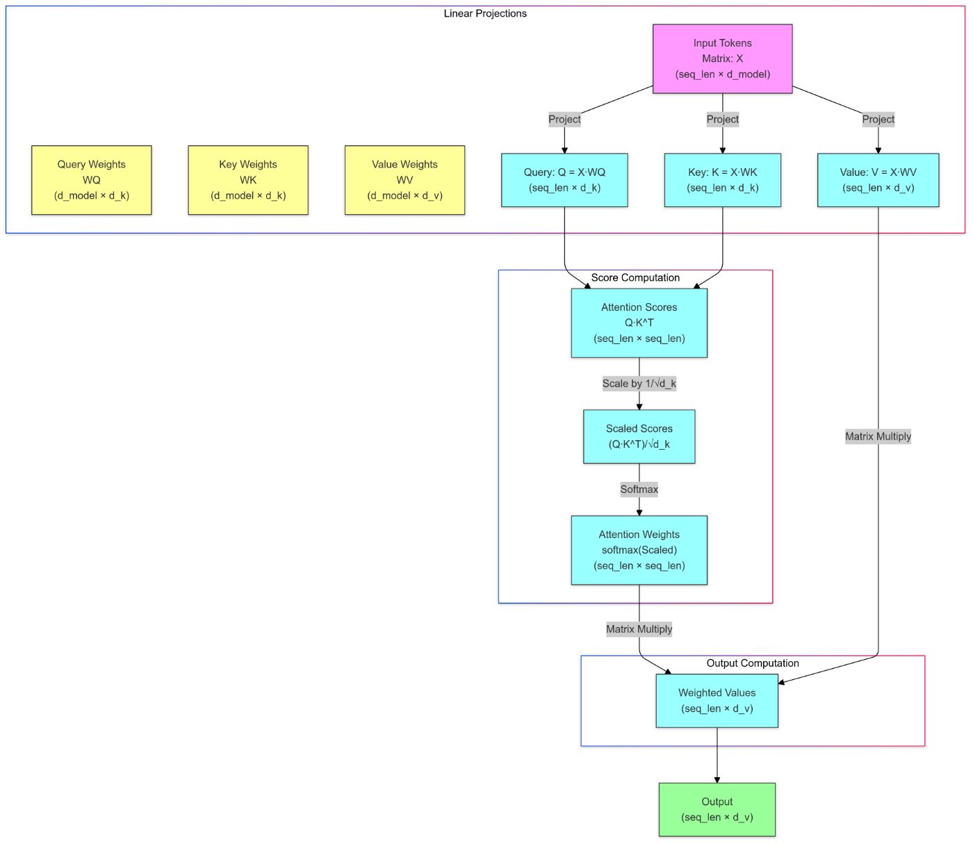
The attention mechanism is a key component of transformer architecture that allows the model to focus on different parts of the input sequence when generating output. It computes a weighted sum of the input representations, where the weights are determined by the relevance of each input token to the current output token being generated. This mechanism enables the model to capture dependencies between tokens, regardless of their distance in the input sequence.
\
The attention mechanism can be computationally expensive, especially for long input sequences, as it requires calculating pairwise interactions between all tokens (O(n^2) complexity). Let’s see it in more step-by-step detail:
\
Input Representation: Each token in the input sequence is represented as a vector, typically using embeddings.
\
Query, Key, Value Vectors: For each token, three vectors are computed: a query vector (
Q_i), a key vector (K_i), and a value vector (V_i). These vectors are derived from the input representations using learned linear transformations.\
Attention Scores: The attention scores are computed by taking the dot product of the query vector of the current token with the key vectors of all previous tokens in the input sequence. This results in a score that indicates how much focus should be placed on each token.
\
Softmax Normalization: The attention scores are then normalized using the softmax function to obtain attention weights, which sum to 1.
\
Weighted Sum: Finally, the output representation for the current token is computed as a weighted sum of the value vectors, using the attention weights.
Multi-Head Attention
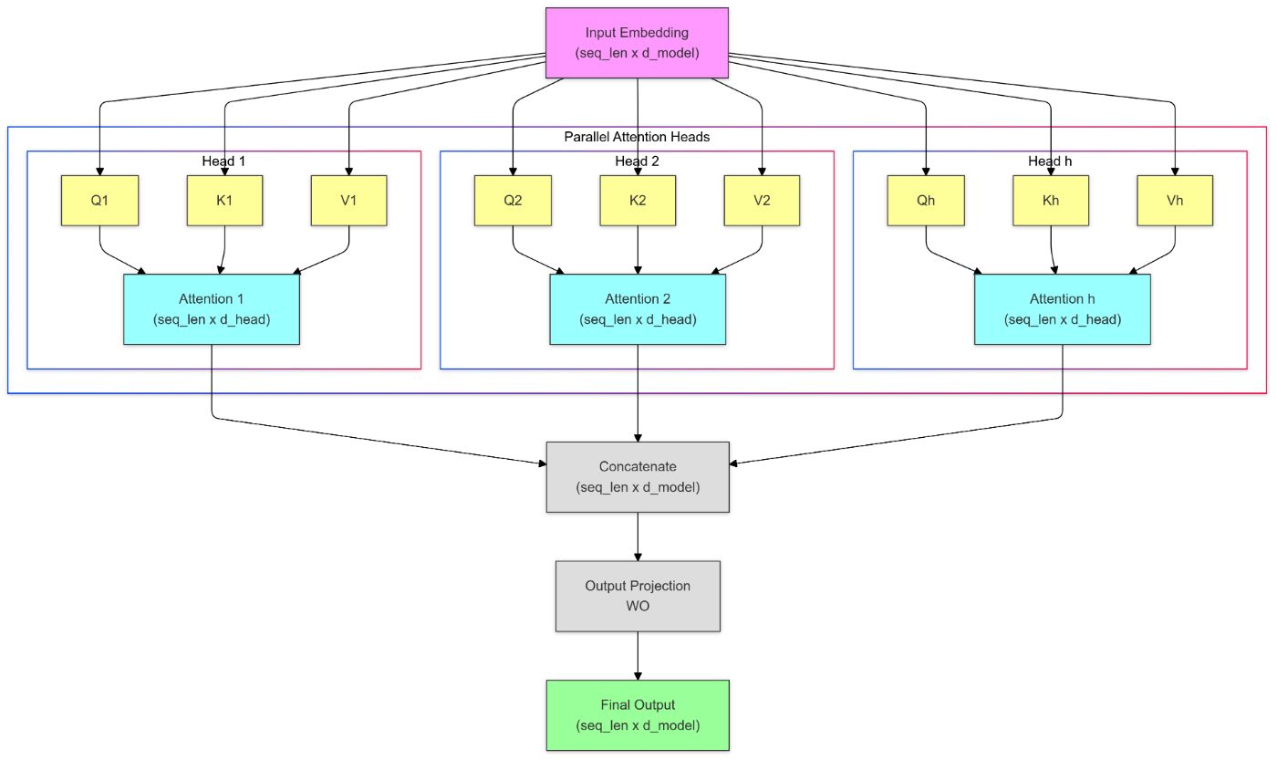
Multi-head attention is an extension of the attention mechanism that allows the model to jointly attend to information from different representation subspaces at different positions. Instead of having a single set of attention weights, multi-head attention computes multiple sets of attention scores in parallel, each with its own learned linear transformations.
\ The outputs of these attention heads are then concatenated and linearly transformed to produce the final output representation.
\ This mechanism enhances the model’s ability to capture diverse relationships and dependencies in the input data, leading to improved performance on various NLP tasks.
Overview of the Inference Computation Process
With an understanding of LLMs and transformer architecture, let’s outline the inference computation process. Inference generates the next $n$ tokens for a given input sequence and can be broken down into two stages:
\
Prefill Stage: In this stage, a forward pass is performed through the model for the input sequence, and key and value representations are computed for each token. These representations are stored for later use in the decoding stage in a K-V cache. Representations of all tokens in each layer are computed in parallel.
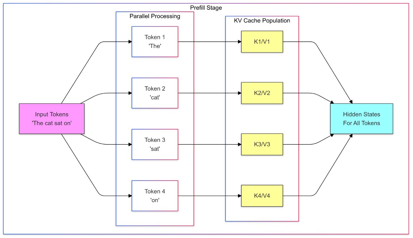
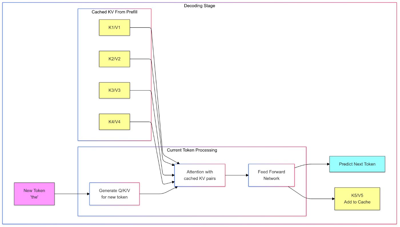
Decoding Stage: In this stage, the model generates the output tokens one at a time in an auto-regressive manner. For each token, the model fetches the key and value representations from the K-V cache stored during the prefill stage, along with the current input token’s query representation to compute the next token in the sequence.
\ This process continues until a stopping criterion is met (e.g., reaching a maximum length or generating an end-of-sequence token). The new key and value representations are stored in the K-V cache for subsequent tokens. In this stage, a token sampling strategy is also applied to determine the next token to generate (e.g., greedy search, beam search, top-k sampling).
Complexity of Inference Computation
For a prefix of length L, embedding size d, and a model with h heads and n layers, the complexity of the inference computation can be analyzed as follows:
Prefill Stage: In the prefill stage, we compute the initial representation for all tokens in the input. The complexity here is:
 Here:
Here:First term
O(L.n .d^2): Represents the feed-forward computation, which processes each token independently across layers. This scales linearly with both sequence length L and the number of layers n.\
Second term
O(L^2. n. h. d): Represents the attention mechanism’s cost. Here, each token interacts with every other token, resulting inL^2complexity for attention calculation per layer. The complexity grows quadratically with sequence length, which can become a major bottleneck for long sequences.\
Decoding Stage: The decoding stage is the autoregressive part, the complexity is:

Here:
Feed-forward computation: For each generated token, we perform feed-forward operations in every layer. Since it’s done for one token at a time (not the whole sequence), the complexity per token is:
O(n.d^2).\
Attention computation with caching: Each new token interacts with the existing sequence through attention, using the previously computed key-value pairs. For each token generated, this attention computation is proportional to the sequence length L , giving:
O(L.n.d .h)\
As we can see, the complexity of the inference computation is influenced by the length of the input sequence (L), the number of layers (n), the number of attention heads (h), and the embedding size (d). This complexity can become a bottleneck in real-time applications, especially when dealing with long input sequences and/or large models.
Importance of K-V Caching
K-V caching is a crucial optimization technique for LLM inference, particularly in the decoding stage. By storing the key and value representations computed during the prefill stage, the model can avoid redundant computations for previously processed tokens.
\ This significantly reduces the computational cost and latency during inference, as the model only needs to compute the attention scores for the new token being generated, rather than recalculating the key and value representations for all tokens in the input sequence.
\ This makes the cost linear with respect to the number of generated tokens, rather than quadratic with respect to the input length.
\ However, K-V caching does require additional memory to store the key and value representations, which can be a trade-off in resource-constrained environments.
Calculations for an Example Model
Let’s calculate the memory requirements for the LLaMA 7B model.
Model Configuration
- Parameters: 7 billion
- Embedding Size (
d_model): 4096 - Number of layers: 32
- Number of attention heads (
d_head): 32 - Head dimension (
d_head): 128 (4096/32) - Max sequence length (L): 2048
- Data type: float16 (2 bytes per element)
Memory Calculation
- Per-Layer Cache Size: For each layer, we need to store both keys and values
Key size per token =
d_head × num_heads= 128 × 32 = 4096 elementsValue size per token =
d_head × num_heads= 128 × 32 = 4096 elementsTotal elements per token per layer = 4096 + 4096 = 8192 elements
\
- Memory Per Layer For Full Sequence: For the full sequence of length L = 2048 tokens
Elements per layer = L × 8192 = 2048 × 8192 = 16,777,216 elements
Memory per layer (in bytes) = 16,777,216 × 2 = 33,554,432 bytes = 33.55 MB
\
- Total KV Cache Memory For All Layers: Since we have $32$ layers
- Total memory = 33.55 × 32 MB = 1073.6 MB
Total Memory Requirement
- Model weights: 7 billion parameters × 2 bytes/parameter = 14 GB
\
- KV Cache Memory: 1073.6 MB
\
- Other memory overhead (e.g., activations, intermediate results): ~1-2 GB
\ Thus, Total memory requirement: 14 GB (model weights) + 1-2 GB (overhead) + 1073.6 MB (KV cache) = 15-16 GB. This calculation gives us an estimate of the memory requirements for the LLaMA 7B model during inference. LLaMA 7B is relatively small compared to models like GPT-3 (175 billion parameters), which would require significantly more memory for both the model weights and the KV cache.
\ Also, when scaled to $m$ concurrent users, resource requirements would be $m$ times higher. Thus, optimization techniques are crucial for deploying large models in resource-constrained environments.
Metrics for Evaluating Inference Optimization
When evaluating the effectiveness of inference optimization techniques, several metrics can be considered:
Pre-fill Latency: The time taken to perform the prefill stage of inference, also called time-to-first-token (TTFT) latency. This metric is crucial for interactive applications where users expect quick responses. Factors like model size, input length, and hardware capabilities can influence this metric.
\
Decoding Latency: The time taken to generate each subsequent token after the prefill stage, also called Inter-Token Latency (ITL). This metric is important for measuring the responsiveness of the model during text generation. For applications like chatbots, low ITL is good, but faster is not always better, as 6-8 tokens per second are often sufficient for human interaction. Affecting factors include K-V cache size, sampling strategy, and hardware.
\
End-to-End Latency: The total time taken from receiving the input to generating the final output. This metric is essential for understanding the overall performance of the inference process and is influenced by prefill, decoding, and other component latencies (e.g. JSON parsing). Affecting factors include model size, input length, and hardware, as well as the efficiency of the entire pipeline.
\
Maximum Request Rate a.k.a QPS (Queries Per Second): The number of inference requests that can be processed per second. This metric is crucial for evaluating the scalability of the model in production environments. Factors like model size, hardware, and optimization techniques can influence QPS. For example, if 15 QPS is served for a P90 latency via 1 GPU, then to serve 300 QPS, 20 GPUs would be needed. Affecting factors include hardware resources, load balancing, and optimization techniques.
\
FLOPS (floating-point operations per second): The number of floating-point operations that the model can perform in a second. This metric is useful for understanding the computational cost of inference and can be used to compare the efficiency of different models and optimization techniques. Affecting factors include model architecture, hardware, and optimization techniques.
Types of Inference Optimization Techniques
We will cover all of these optimization in future post of the series.
- Model Architecture Optimization: Modifying the model architecture to improve inference efficiency, such as reducing the number of layers or attention heads, or using more efficient attention mechanisms (e.g., sparse attention).
\
System Optimization: Optimizing the underlying hardware and software infrastructure, such as using specialized hardware (e.g., TPUs, GPUs) or optimizing the software stack (e.g., using efficient libraries and frameworks). It can be broken down into:
\
Memory management: Efficiently managing memory usage to reduce overhead and improve performance.
Efficient Computation: Leveraging parallelism and optimizing computation to reduce latency.
Batching: Processing multiple requests simultaneously to improve throughput.
Scheduling: Efficiently scheduling tasks to maximize resource utilization.
\
Model Compressions: Techniques like quantization, pruning, and distillation can be used to reduce the size of the model and improve inference speed without significantly sacrificing performance.
\
Algorithm Optimization: Improving the algorithms used for inference, such as using more efficient sampling strategies or optimizing the attention mechanism. E.g. Speculative decoding, which allows the model to generate multiple tokens in parallel, can significantly reduce decoding latency.

\
Conclusion
In this post, we provided an overview of LLM inference, its importance, and the challenges associated with it. We also outlined the key problem formulations that will guide our exploration of optimization techniques in subsequent posts.
\ By understanding the intricacies of LLM inference and the factors that influence its performance, we can better appreciate the significance of optimization techniques in making LLMs more practical for real-world applications. In the next post, we will delve deeper into specific optimization techniques and their implementations, focusing on reducing latency and resource consumption while maintaining model performance.
References
\
This content originally appeared on HackerNoon and was authored by Ravi Mandliya
Ravi Mandliya | Sciencx (2024-11-04T22:04:58+00:00) Primer on Large Language Model (LLM) Inference Optimizations: 1. Background and Problem Formulation. Retrieved from https://www.scien.cx/2024/11/04/primer-on-large-language-model-llm-inference-optimizations-1-background-and-problem-formulation/
Please log in to upload a file.
There are no updates yet.
Click the Upload button above to add an update.
