This content originally appeared on Level Up Coding - Medium and was authored by Tirendaz Academy
Machine learning and deep learning with TensorFlow and Keras
With the development of artificial intelligence, previously unsolvable problems could be solved. In this article, I will introduce deep learning with TensorFlow.

What is Deep Learning?
In recent years, data production has increased with the development of the internet and technology. Machine learning techniques are used to extract information from data. But machine learning techniques were insufficient to analyze big data.
Deep learning techniques have been used to find patterns in big data in recent years. Most of the deep learning techniques had been discovered before, but these techniques were not fully utilized due to scarcity of data and lack of hardware.
In recent years, with the increase in data and the development of technology, humanoid tasks have been performed with deep learning.
What is TensorFlow ? & How to Install?
TensorFlow is an open-source machine learning platform developed by Google. Deep learning analysis can be done easily with TensorFlow. It can be used in PyTorch developed by Facebook for deep learning. But TensorFlow is used more for end-to-end projects.
To install TensorFlow, you first need to install Python. You can install Python on your computer from here.
Installed in pip when installing Python. pip is a package manager for installing and managing third-party Python packages. To install TensorFlow, you need to install the newest version of pip. You can use the following codes to update pip.
pip install — upgrade pip
Virtual Environment Installation
Sometimes you can work with multiple projects at the same time. You may want to use different libraries for each project. By using a virtual environment, you can prevent these libraries from colliding.
With the virtual environment, you can separate the library you use for each project. So your libraries won’t conflict. You can use various methods such as pipenv or venv to set up a virtual environment.
To set up the virtual environment, let’s open the command line first and create a new directory by typing the commands below and go to this directory.
mkdir tf_project
cd tf_project
I created the project working directory. Let’s set up a new virtual environment in this directory with venv.
python3 -m venv tensorflow
With these commands, the latest version of Python is loaded by default. After the virtual environment is loaded, it is necessary to activate this environment. You can use the command below for this.
source env / bin / activate
You can understand that the virtual environment is active from the name of the virtual environment at the beginning of the line.
You can use pip to upload packages or libraries to this virtual environment. First, update the pip in this virtual environment so that the latest versions of the libraries you will install are installed.
pip install — upgrade pip
You can use the commands below to see the installed packages in the virtual environment.
pip list
Let’s set up TensorFlow with the pip command.
pip install tensorflow
You can use various editors such as etc code, sublime text to write the codes. Jupyter Notebook is often used in data science projects because it visualizes data well. Let’s install this editor in our virtual environment.
pip install notebook
To start Jupyter Notebook, simply type the following command on the command line.
jupyter notebook
After Jupyter Notebook opens, create a new Python file. To work with TensorFlow, you have to import it.
Let’s import TensorFlow with the tf.
import tensorflow as tf
If you do not get any errors when you run this command, then TensorFlow has been installed without any errors.
Colab
You can use Colab to work with TensorFlow. Colab is a cloud service similar to Jupyter Notebook offered by google. Libraries such as TensorFlow, Pandas, NumPy are installed in Colab. You can use these libraries by importing them directly.
To use Colab, you can go to this address. Do not forget to click on CONNECT in the upper right corner while working in Colab. First, let’s import TensorFlow with the tf.
import tensorflow as tf
Deep Neural Networks
Artificial neural networks are a technique that emerged to find patterns in data by imitating the human brain. Artificial neural networks have been successful in solving linear problems, but they have failed to solve non-linear problems. Hidden layers have been added to artificial neural networks to solve non-linear problems.
Artificial neural networks with more than one hidden layer are called deep neural networks.
Extracting information from data using the deep neural networks technique is called deep learning. With deep learning, previously unsolvable problems are solved such as
- Image classification
- Voice recognition
- Machine translation
- Assistant assistants like Siri and Alex
- Driverless cars
- Convert speech to sound

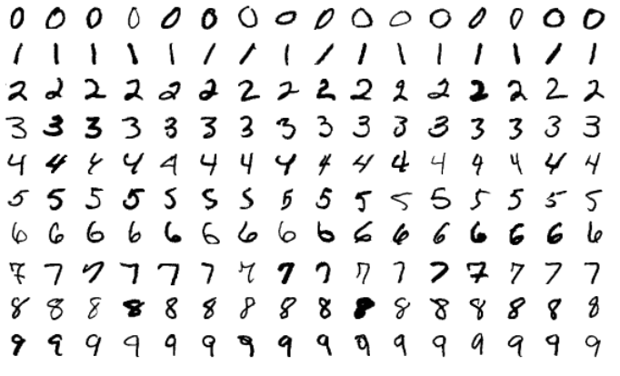
Let’s use the mnist dataset to show deep neural networks. This dataset contains grayscale 0 to 9 digit images in 28 * 28 pixels. This dataset contains 60,000 training pictures and 10,000 test pictures. You can think of analyzing the MNIST dataset as the “Hello World” of deep learning.
Let’s first import this data set.
mnist = tf.keras.datasets.mnist
Let’s split this dataset into training and testing. Remember, the model is established with the training data, and the model is evaluated with the test data.
(x_train, y_train), (x_test, y_test) = mnist.load_data ()

Images are encoded as a NumPy array. Labels are numbers from 0 to 9. Let’s look at the structure of the data sets.
print (x_train.shape)
print (x_test.shape)

Scaling data in deep learning analyzes both speeds up the training of the network and increases the accuracy of the network. Let’s scale the data between 0 and 1.
x_train, x_test = x_train / 255.0, x_test / 255.0
Now we can start building the neural network. You can create the neural network as a sequence of layers. You can think of Layer as a filter that extracts information from data. I will use the Sequential technique for this analysis.
model = tf.keras.models.Sequential ([
   tf.keras.layers.Flatten (input_shape = (28, 28)), (1)
   tf.keras.layers.Dense (128, activation = ‘relu’), (2)
   tf.keras.layers.Dropout (0.2),                    (3)
   tf.keras.layers.Dense (10)                        (4)
])
(1) The first layer is the input layer. Flatten is used to flatten the input.
(2) The second layer is Dense layer. Dense layer is called fully connected. All neurons in this layer are connected to all previous neurons. I determined the number of neurons in this layer as 128 and the activation function as relu (rectified linear unit). Layers can only learn linear transformations of inputs. Activation functions are used to learn more complex patterns in the data. It has activation functions such as elu, tanh, but mostly relu activation function is used in deep learning analysis. The relu function takes negative values to 0.
(3) If the model shows good performance in training data but poor performance in test data, an overfitting problem arises. The regularization technique is used to overcome the overfitting problem. There are regularization techniques such as L1 and L2. Here I used the Dropout technique.
Dropout is a regularization technique used for neural networks. When dropout is applied to a layer, a random part of the output is dropped during training. Thus, excessive memorization of the model is prevented. I scale down the output by the dropout rate. Here, I scale by 0.2.
(4) The last layer is the output layer. I put 10 on this layer because there are 10 classes in the result variable.
So I built a neural network architecture. In order to prepare the neural network for training, it is necessary to compile the model. Three arguments are specified while compiling the model.
model.compile (optimizer = ‘man’, (1)
    loss = tf.keras.losses.SparseCategoricalCrossentropy(
             from_logits = True), (2)
    metrics = [‘accuracy’]        (3)
)
(1) The loss function measures the performance of the neural network over training data. It does this by comparing the estimate of the neural network with the actual value. You can use SparseCategoricalCrossentropy as a loss function when you have two or more classes. If you have coded tags with one-hot, you can use the CategoricalCrossentropy loss.
(2) Optimizer updates the weights used in the neural network according to the value of the loss function. There are various optimizer functions such as RMSProp, SGD. The Adam (adaptive moment estimation) optimizer has become particularly popular in recent years. This algorithm is an extension of stochastic gradient descent.
(3) The Metrics argument is used to see the performance of the neural network. I used the accuracy metric for the analysis classification problem.
So far I have built the architecture of the model and compiled the model using the compile method. Now the model is ready for training. Let’s train the neural network by calling the fit method.
model.fit(x_train, y_train, epochs = 5)

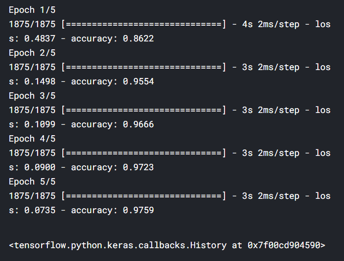
Each iteration on training data is called an epoch. At each iteration, the neural network updates the weights according to the loss function.
During the training, the loss and accuracy of the network were written on the screen. The accuracy of the model on training data is about 98 percent. After training the model, evaluate () method is used to evaluate the performance of the model on the test set.
model.evaluate(x_test, y_test)

Thus, the accuracy of the model on the training data was written on the screen. The accuracy of the model on test data is about 98 percent. So we built the first neural network. You can find the notebook I used in this article here.
Thank you for reading my article. I explained the following topics in this article;
- What is deep learning?
- How to install TensorFlow?
- Training and evaluating a deep learning model with TensorFlow
The following articles may also be of interest to you.
- Data Visualization with Pandas and Seaborn ?
- PRACTICAL DATA ANALYSIS with PANDAS
- How to Fix Missing Data in Pandas
Introduction to Deep Learning with TensorFlow 2 was originally published in Level Up Coding on Medium, where people are continuing the conversation by highlighting and responding to this story.
This content originally appeared on Level Up Coding - Medium and was authored by Tirendaz Academy
Tirendaz Academy | Sciencx (2021-04-15T13:24:20+00:00) Introduction to Deep Learning with TensorFlow 2. Retrieved from https://www.scien.cx/2021/04/15/introduction-to-deep-learning-with-tensorflow-2/
Please log in to upload a file.
There are no updates yet.
Click the Upload button above to add an update.
