This content originally appeared on HackerNoon and was authored by Reinforcement Technology Advancements
:::info Authors:
(1) J. Quetzalcóatl Toledo-Marín, University of British Columbia, BC Children’s Hospital Research Institute Vancouver BC, Canada (Email: j.toledo.mx@gmail.com);
(2) James A. Glazier, Biocomplexity Institute and Department of Intelligent Systems Engineering, Indiana University, Bloomington, IN 47408, USA (Email: jaglazier@gmail.com);
(3) Geoffrey Fox, University of Virginia, Computer Science and Biocomplexity Institute, 994 Research Park Blvd, Charlottesville, Virginia, 22911, USA (Email: gcfexchange@gmail.com).
:::
Table of Links
3 Results
3.1 Performance for different loss functions and data set sizes
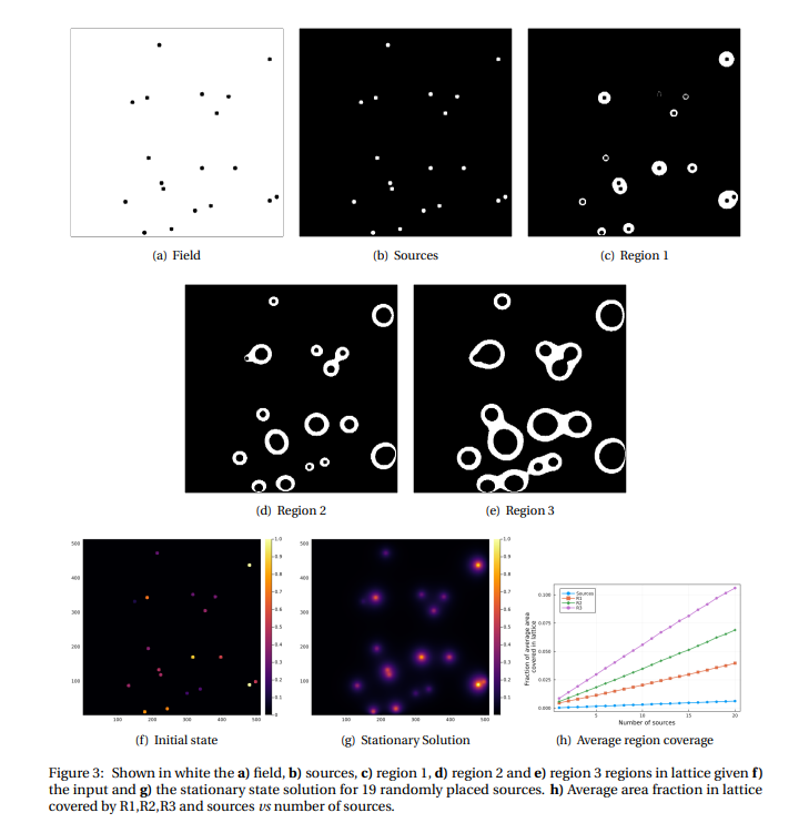
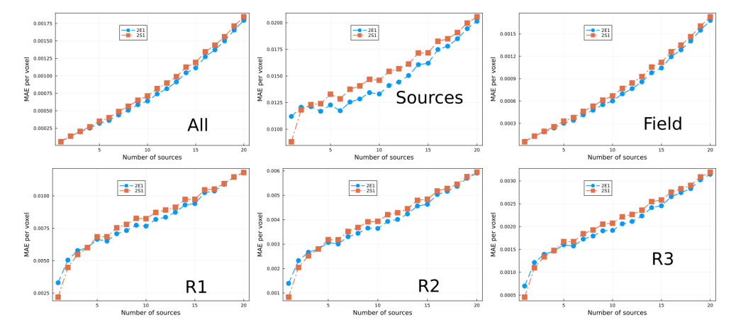
In this section we present the performance results of each of the models we trained. To this end, we use the MAE between prediction and target for each model. In general, models with good performance may not necessarily perform well in predicting sources and/or the field close to sources. In addition to computing the MAE on the whole lattice, we also measured the MAE in different regions in the lattice as shown in Fig. 3. Filtering field and sources can be done using the initial state, while regions R1, R2 and R3 correspond to pixel values in [0.2,1], [0.1,0.2] and [0.05,0.1], respectively. We compare the effects of different loss functions and different data set sizes. We validate all of our models using the same test set composed by 80k tuples (i.e., input and target).
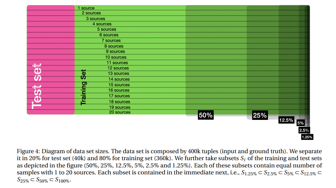
\ In general, there are three main factors that contribute to the performance difference between different models, namely, the data set size, the loss function and the pseudo-stochasticity when training the model (weights initialization, minibatch parsing, etc). We found that the factor that contributes the most to performance is the data set size. For clarity purposes, we present our results by clustering models by data size trained on. We trained models using 1.25%,2.5%,5%,12.5%,25%,50% and 100% of the training set. In every training set partition we selected an equal number of tuples per number of sources. Additionally, the data set with 1.25% is a subset of the data set with 2.5% which is a subset of the data set with 5% and hence forth as depicted in Fig. 4. After training each model, we evaluated the performance on the test set per number of sources (see Fig. 4). We tagged each model with a code which references the data set size used, the prefactor used, whether it was trained with MAE, MSE, Huber or inverse Huber and, in some case, we reference in the naming code the hyperparameters used. For instance, model 40E1 was trained with 1/40 = 2.5% of the data set, an exponential prefactor and MAE while 80EIH was trained using 1/80 = 1.25% of the data set, exponential prefactor and inverse Huber.
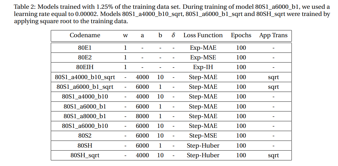
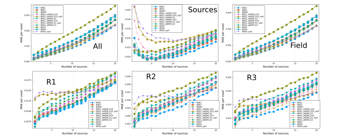
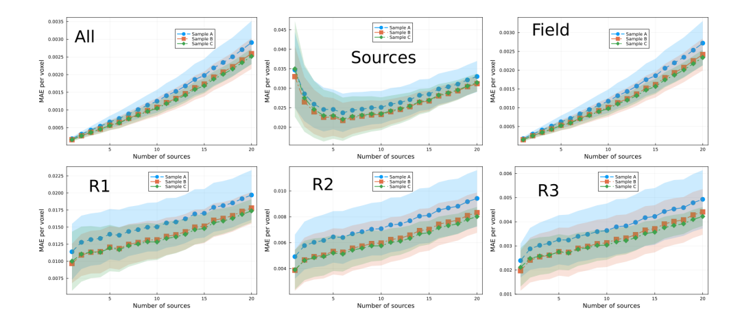
\ In Fig. 5 we show the MAE for models trained with 1.25% of the data set. The hyperparameter selected for each model are displayed in Table 2. There are a number of features to highlight from Fig. 5. First, the largest absolute error occurs at the sources and decreases as one moves away from the sources. In addition, the error increases monotonically with the number of sources. Interestingly, as the number of sources increases, the error at the sources decreases rapidly and then increases slow and steadily. Most models performed quite similar, but overall model 80E1 performed best. However, the difference in performance is not significant as we will discuss next.
\ To assess the amplitude of fluctuations in performance due to stochasticity from initialization and training of the models, we trained three sets of five models each. All models were trained using the same hyperparameters. Each
\
\
\ set was trained with a 1.25% data set, such that there was no overlap between the data sets. In Fig. 6 we show the average performance and standard deviation (in shadow) per set. Notice that there is no significant improvement between sets. Furthermore, the fluctuations per set are large enough to conclude that the different performances between the different models in Fig. 5 can be attributed to fluctuations.
\
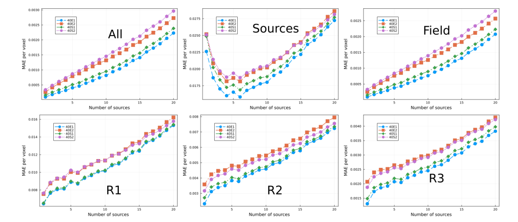
\ In Fig. 7 we show the MAE for models trained with 2.5% of the data set. The hyperparameter selected for each model are displayed in Table 3. Model 40E1, which was trained using the exponential weight MAE loss function, performed best in all the lattice regions and for all number of sources. However, notice that the model with the second best performance, model 40S1, was trained using the step-weighed MAE, while what the two worst two models have in common is that both were trained using MSE. Furthermore, the largest difference in performance between the best and the worst model, which happens in the sources, relative to the error is ≈ 0.2. This suggests the different performance in models can be attributed to fluctuations and not necessarily the effect of the loss function. On the other hand, it was found that, in general, the performance decreases as the number of sources increases. As noted previously, in the case of the sources the performance first decreases, reaching a minimum around 5 sources and it then increases with the number of sources. The appearance of a minimum in performance is a feature that we will come across throughout the present paper and we leave the discussion for later.
\

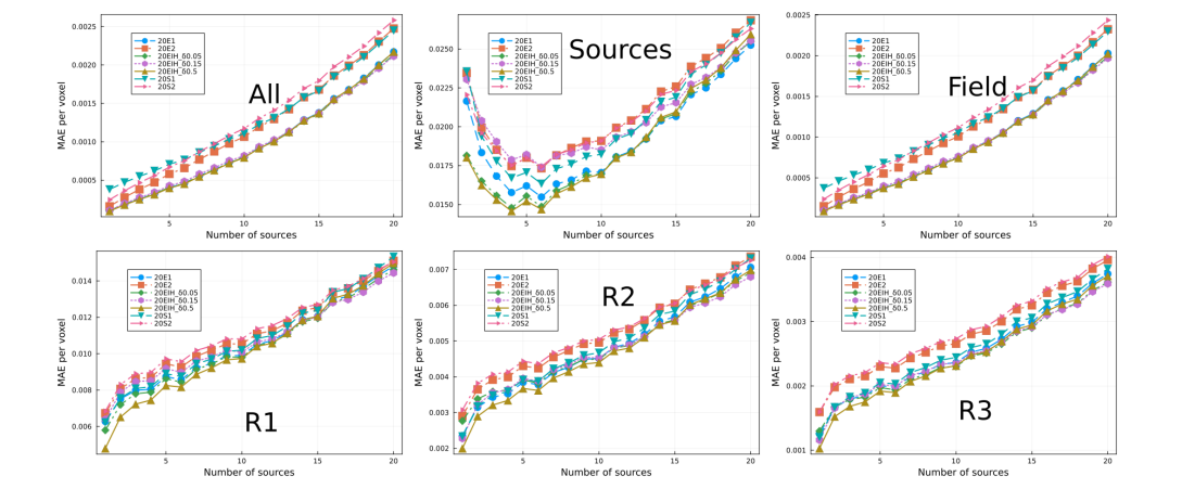
\ In Fig. 8 we show the MAE for models trained with 5% of the data set. The hyperparameter selected for each model are displayed in Table 4. Notice that the same general trends discussed previously also holds in this case. In particular, models 20EIH-# performed best, which were trained using the exponential weight inverse Huber loss function. On the other hand, model 20E2 had the worst performance. To assess the amplitude of fluctuations in performance due to stochasticity from initialization and training of the models, we trained two sets of five models
\
\
\

\
\
\
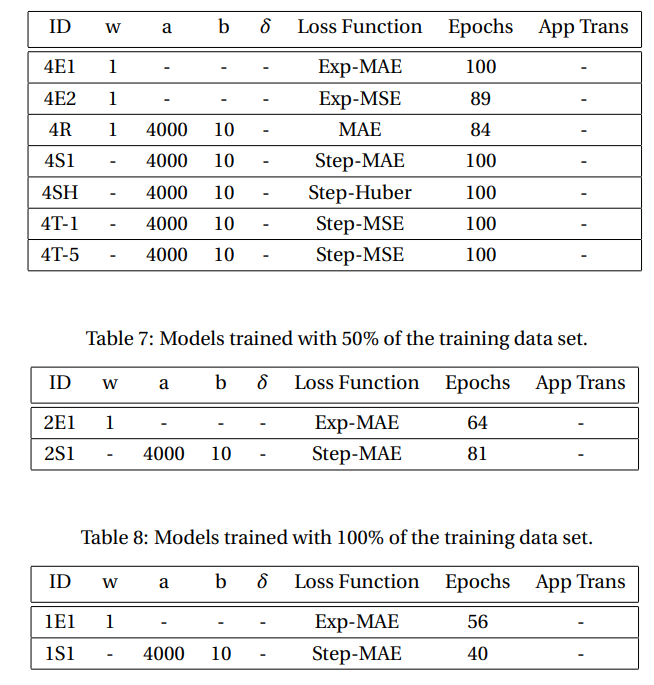
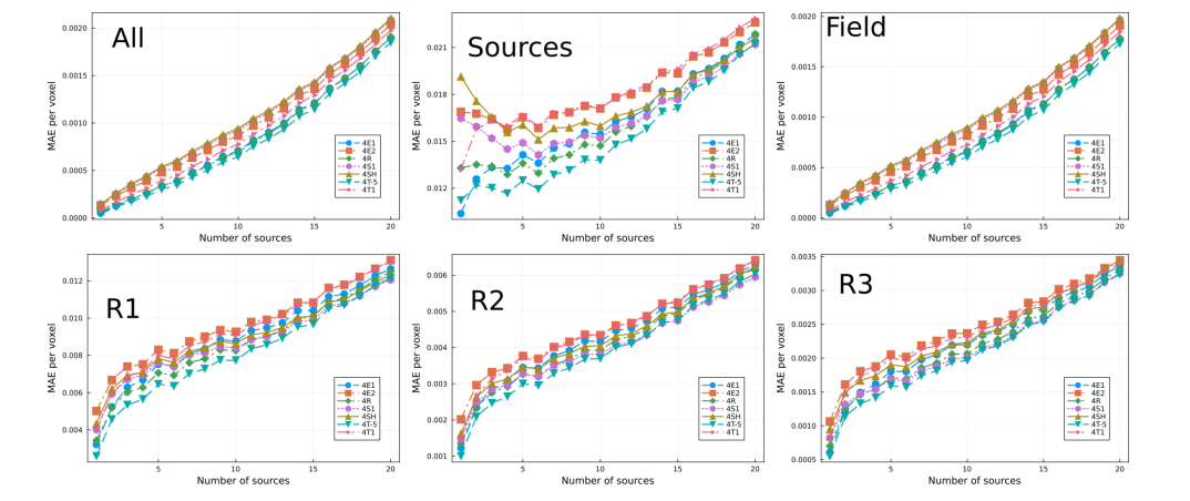
\ Table 6: Models trained with 25% of the training data set. Model 4E2-2 was trained adding Gaussian noise w/ standard deviation equal to 0.01 on the groundtruth. In training model 4R, each epoch selected either step or exp prefactor randomly with probability 0.8 for the former and 0.2 for the latter. In training model 4T-1, the loss function toggled between step and exp prefactor, starting with exp. In training model 4T-5, the loss function toggled between step and exp prefactor every 5 epochs.
\
\
\
\
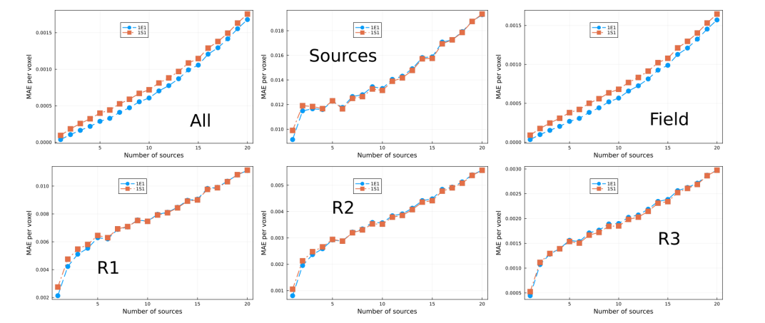
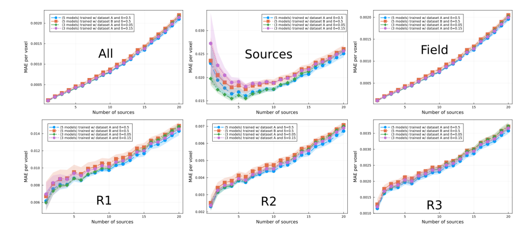
\ each. All models were trained using the same hyperparameters. Each set was trained with a 5% data set, such that there was no overlap between the training sets. We also trained two sets more composed by 3 models each, using different δ-hyperparameter. In Fig. 9 we show the average performance and standard deviation (in shadow) per set. Notice that there is no significant improvement between sets. However, the fluctuations per set have reduced quite substantially compared to the 1.25% case shown in Fig. 6 and discussed previously. In this regard, the different performances between the different models in Fig. 8 can be attributed to some extent to fluctuations, however notice that model 20E2 can be taken as an outlier.
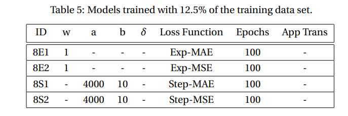
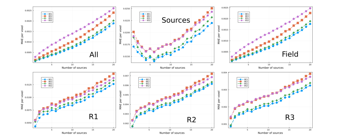
\ We trained multiple models using 12%, 25%, 50% and 100% of the data set. The models hyperparameters are specified in Tables 5, 6, 7 and 8, respectively. The performances are shown in Figs. 10, 11, 12 and 13, respectively. A repeating feature is that the error increases with the number of sources in all cases, as discussed previously. Moreover, models trained using the exp prefactor typically outperform the rest. We also trained a model, 4R, that each epoch randomly selects between exp-prefactor and step-prefactor with probability 0.2 and 0.8, respectively. We also trained two models, 4T-1 and 4T-5, that toggle between step- and exp-prefactor every 1 and 5 epochs, respectively. Notice that models 4R and 4T-5 outperform the rest, including 4E1. The rationale behind models 4Tand 4R is that perturbing the model over the loss function landscape, via toggling or randomly choosing between the loss functions, can help the model find a lower local minimum. In the case of 50% and 100% data set size, we only trained two models per data set size as we wanted to compare performance between step- and exp-prefactor. The exponential weighing prefactor show better performance in all regions of the lattice, as shown in Figs. 12 and 13.
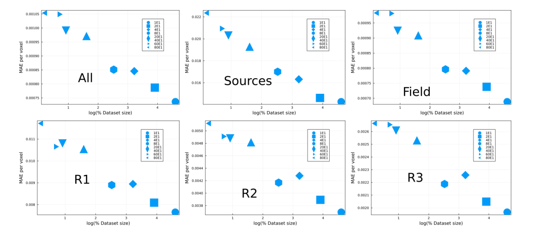
\ In the previous the different performances for different data set size and different loss functions were shown and discussed. We showed that increasing the data set size decreases the performance fluctuations. We also showed that, in general, different loss functions yield similar performance. However, increasing the data set size improves the model performance. In Fig. 14 we show the performance of models trained with different data set size and with the same loss function, namely, exponential-weighed MAE. Notice the performance has a logarithmic dependence on the training set size. The main takeaways are, first, models trained with exponential prefactor and MAE consistently show better performance; second, changing loss functions between epochs can have a positive effect in performance as seen by models 4R and 4T-5; third, as expected the error decreases with the training set size; fourth, as the training size increases the performance increases but the rate decreases. The later is surprising, because the high dimensionality of the problem means that even our largest training set significantly undersamples the space of possible configurations. This saturation points to a possible fundamental limit in the ability of the encoder-decoder network to solve the diffusion problem and suggests that other networks might be more effective.
\
3.2 Inference
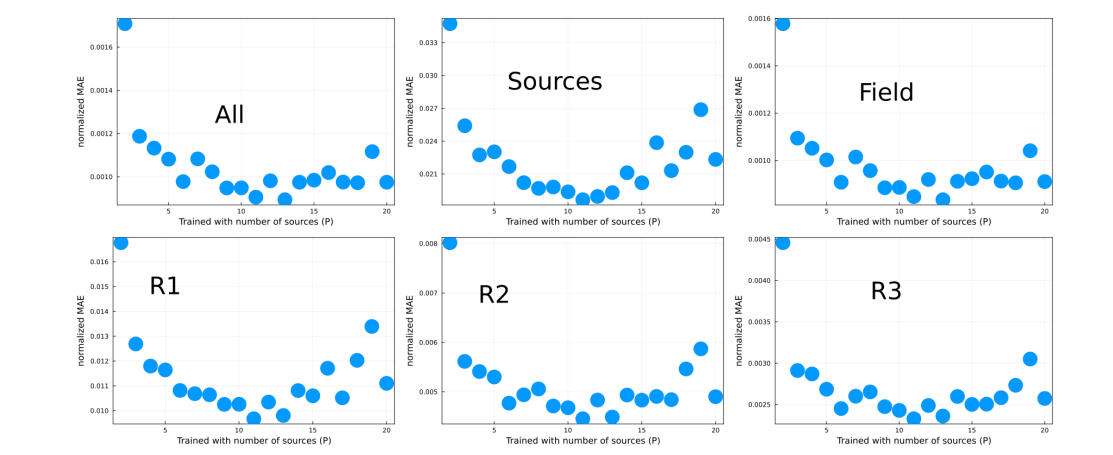
In this section we present and discuss the results for prediction by inference. While in the previous section we focused on performance for different data set size, here we study performance of models trained on a data set with a fixed number of sources. In this sense, we look at how well a model performs when given an input with an arbitrary number of sources different to the number of sources the model was trained on. This is particularly relevant since, by brute estimation, the configurational space is considerably large and exponentially dependent on the number of sources, however, by taking into account the configurational space symmetries one could construct the training set where the number of samples is depend on the number of sources. We found that there is an optimum, i.e., models trained on a fixed and different number of sources perform differently
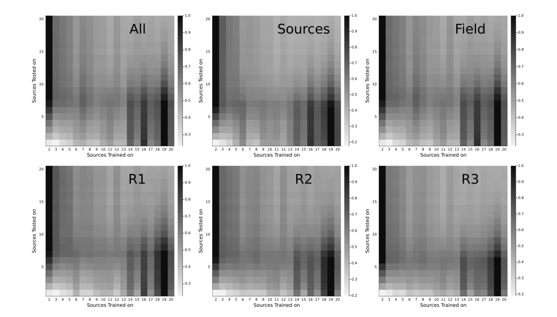
\ We trained 20 models on each of the 20 data sets one-on-one. Each model was trained for 100 epochs and using the exponentially weighed MAE as the loss function. To measure the inference prediction, we test the prediction of each model over each of the 20 test sets. Fig. 16 shows a density plot of the normalized MAE for different regions in the lattice. The normalization is per row, i.e., for a fixed number of sources tested on (Y axis), each row yields the normalized MAE corresponding to each of the 19 models trained using a fixed number of sources (we have not included the model trained using 1 source as the MAE is an order of magnitude larger). These plots show that there is not a model that outperforms the rest for all test sets, rather models trained with ∼ 10−12 perform better.
\ We have averaged each of the non-normalized rows in Fig. 16 and we have plotted the values in Fig. 17. The model that yields the minimum error will depend on the region in the lattice we are considering, yet overall the optimum lies in models trained between 10 and 13 sources. The previous results suggest that the different configurations obtained from considering 10 to 13 sources in a lattice is sufficient to extrapolate to the different configuration that can arise from considering more sources. We can understand this in the following manner. Notice that what the model is learning is the field generated by the superposition of sources at different relative distances. In this regard, a model trained using a data set with a small number of sources will not have a large number of sources clustered and, hence, will never learn the field generated from a large number of sources. On the other hand, a data set with a large number of sources will most likely have a large number of clustered sources and lack small clusters of sources and, thus, a model trained using this data set will not learn the field generated from a few close sources. The data sets with number of sources around 12 are such that contain different clusters as depicted in Fig. 15. The results in Figs. 16 and 17 are in fact suggesting redundancy in the data set, i.e., a better curated data set would be comprised by different data set sizes dependent upon the number of sources.
\

\
\
\
:::info This paper is available on arxiv under CC 4.0 license.
:::
\
This content originally appeared on HackerNoon and was authored by Reinforcement Technology Advancements
Reinforcement Technology Advancements | Sciencx (2024-06-21T07:30:16+00:00) Understanding Factors Affecting Neural Network Performance in Diffusion Prediction. Retrieved from https://www.scien.cx/2024/06/21/understanding-factors-affecting-neural-network-performance-in-diffusion-prediction/
Please log in to upload a file.
There are no updates yet.
Click the Upload button above to add an update.
