
This content originally appeared on Level Up Coding - Medium and was authored by CyCoderX

Master Data Analysis and Data Science Techniques Using Python with Car Sales Data
Introduction
In our data-driven world, extracting meaningful insights from information is crucial for software developers. Python, with its robust ecosystem, has become a powerhouse for data analysis and statistical computing. This guide will walk you through using Python to derive statistics from data, enabling you to make informed decisions and uncover hidden patterns in your datasets.
This comprehensive guide caters to both seasoned developers and tech enthusiasts eager to explore data science. We’ll cover everything from basic statistical measures to advanced analytical techniques, using real-world examples and clear, commented code snippets. By leveraging popular libraries like pandas, numpy, matplotlib, and seaborn, you’ll gain practical skills in statistical analysis with Python.
Throughout this journey, we’ll be leveraging popular Python libraries such as pandas for data manipulation, numpy for numerical computing, and matplotlib and seaborn for data visualization. By the end of this article, you’ll have a solid foundation in using Python for statistical analysis, enabling you to:
- Efficiently import and explore diverse datasets
- Calculate and interpret basic statistical measures
- Create insightful visualizations to communicate your findings
- Perform advanced statistical analyses to uncover deeper insights
- Apply these skills to real-world scenarios and challenges
So, let’s embark on this exciting journey into the world of data statistics with Python. Whether you’re analyzing user behavior in a web application, optimizing algorithms, or diving into scientific research, the skills you’ll learn here will prove invaluable in your career as a software developer or data enthusiast.
Did you know that you can clap up to 50 times per article? Well now you do! Please consider helping me out by clapping and following me! 😊
Your engagement — whether through claps, comments, or following me — fuels my passion for creating and sharing more informative content.
Additionally, if you’re interested in more Python, SQL or similar content content, please consider following me.
Database SQL Sagas By CyCoderX
Setting Up the Environment
Before we dive into statistical analysis with Python, it’s crucial to set up a proper development environment. This section will guide you through the process of installing Python and the necessary libraries for data analysis.
1. Installing Python
If you haven’t already, download and install Python from the official website (https://www.python.org/). We recommend using Python 3.8 or later for this tutorial.
2. Setting up a Virtual Environment
It’s a best practice to use virtual environments for Python projects. This isolates your project dependencies from other projects and system-wide packages.
# Create a new virtual environment
python -m venv stats_env

# Activate the virtual environment
# On Windows:
# stats_env\Scripts\activate
# On macOS and Linux:
# source stats_env/bin/activate
3. Installing Required Libraries
We’ll be using several libraries throughout this tutorial. Install them using pip, Python’s package installer:
pip install numpy pandas matplotlib seaborn scipy statsmodels
4. Verifying the Installation
Let’s create a simple Python script to verify that everything is installed correctly:
import numpy as np
import pandas as pd
import matplotlib.pyplot as plt
import seaborn as sns
from scipy import stats
import statsmodels.api as sm

print("NumPy version:", np.__version__)
print("Pandas version:", pd.__version__)
print("Matplotlib version:", plt.__version__)
print("Seaborn version:", sns.__version__)
print("SciPy version:", stats.__version__)
print("Statsmodels version:", sm.__version__)

# Create a simple plot to test visualization libraries
x = np.linspace(0, 10, 100)
y = np.sin(x)
plt.plot(x, y)
plt.title("Test Plot: Sine Wave")
plt.show()
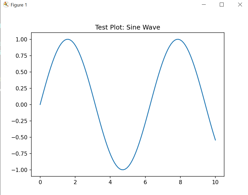
Run this script. If it executes without errors and displays version information along with a sine wave plot, your environment is set up correctly.
5. Integrated Development Environment (IDE)
While you can use any text editor for Python development, an IDE can significantly enhance your productivity. Some popular options include:
- PyCharm: A full-featured IDE with excellent debugging capabilities.
- Visual Studio Code: A lightweight, extensible editor with great Python support.
- Jupyter Notebook: An interactive environment perfect for data analysis and visualization.
Choose the one that best fits your workflow. For this tutorial, we’ll use standard Python scripts, but the code can be easily adapted to Jupyter Notebooks if you prefer.
With your environment set up, you’re now ready to begin your journey into statistical analysis with Python. In the next section, we’ll start by importing and exploring our first dataset.
Clean Code in Python: Good vs. Bad Practices Examples
Looking to enhance your Python skills? Delve into practical examples of good versus bad coding practices in my article on Clean Code in Python, and master the fundamentals of Python classes and objects for a comprehensive understanding of programming principles.
Python Classes and Objects: An Essential Introduction
Importing and Exploring Data
Before we can perform any statistical analysis, we need to import our data and get a good understanding of its structure and content. In this section, we’ll learn how to load data into Python using pandas and perform initial exploratory data analysis.
Importing Data
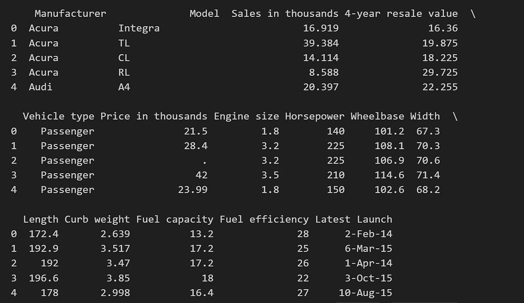
For this tutorial, we’ll use a dataset containing information about used cars. Let’s start by importing it using pandas:
Use this dataset: https://github.com/chandanverma07/DataSets/blob/master/Car_sales.csv
import pandas as pd
import numpy as np
import matplotlib.pyplot as plt
import seaborn as sns

# Load the dataset
df = pd.read_csv("Car_sales.csv")

# Display the first few rows
print(df.head())
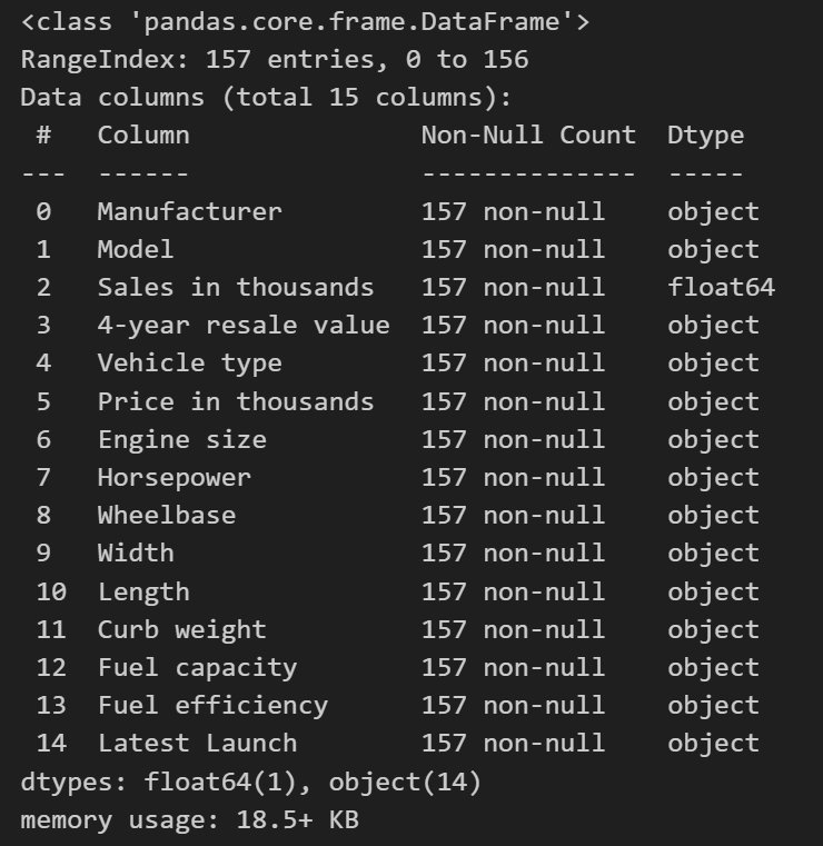
Understanding the Dataset Structure
Let’s examine the structure of our dataset:
# Get basic information about the dataset
print(df.info())
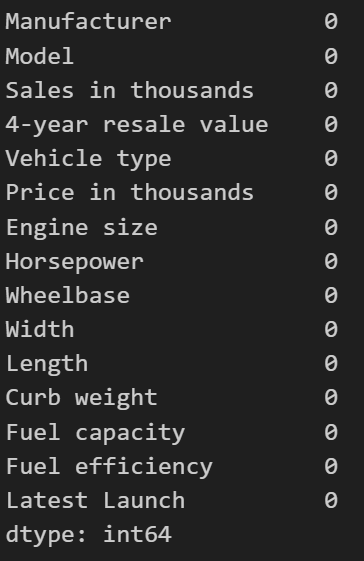
# Check for missing values
print(df.isnull().sum())
Seems we will need to change the type of some columns:
But it seems we do not have duplicate data:
Master Python Enum Module: A Comprehensive Guide
Your engagement, whether through claps, comments, or following me, fuels my passion for creating and sharing more informative content.
If you’re interested in more SQL or Python content, please consider following me. Alternatively, you can click here to check out my Python list on Medium.
Elevate Your Data Analysis Skills with Pandas
Data Cleaning and Preprocessing
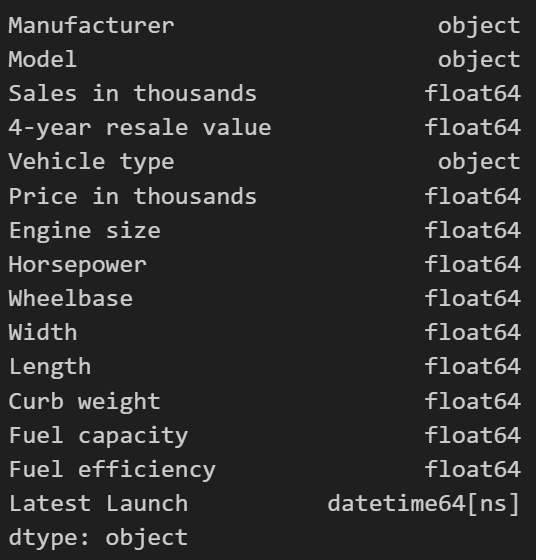
Next, we will need to identify the columns that need type conversion. Specifically:
- Columns like “4-year resale value”, “Price in thousands”, “Engine size”, “Horsepower”, “Wheelbase”, “Width”, “Length”, “Curb weight”, “Fuel capacity”, and “Fuel efficiency” should be converted to numeric types.
- The “Latest Launch” column should be converted to datetime type.
# Convert columns to numeric types
numeric_columns = [
    '4-year resale value', 'Price in thousands', 'Engine size',
    'Horsepower', 'Wheelbase', 'Width', 'Length', 'Curb weight',
    'Fuel capacity', 'Fuel efficiency'
]

for col in numeric_columns:
    df[col] = pd.to_numeric(df[col], errors='coerce')

# Convert 'Latest Launch' to datetime type
df['Latest Launch'] = pd.to_datetime(df['Latest Launch'], errors='coerce')

# Display the data types to confirm changes
df.dtypes
Output:
Displaying statistics:
df.describe()

Did you know I have articles on Data Science using Python and NumPy? These resources cover essential concepts, practical examples, and hands-on exercises. 📊🐍
Exploring Relationships in the Data
Now that our data is prepared, let’s explore some relationships:
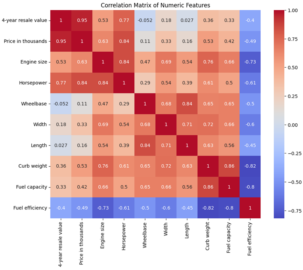
# Calculate the correlation matrix
correlation_matrix = df[numeric_columns].corr()
# Plot the heatmap
plt.figure(figsize=(10, 8))
sns.heatmap(correlation_matrix, annot=True, cmap='coolwarm')
plt.title('Correlation Matrix of Numeric Features')
plt.show()
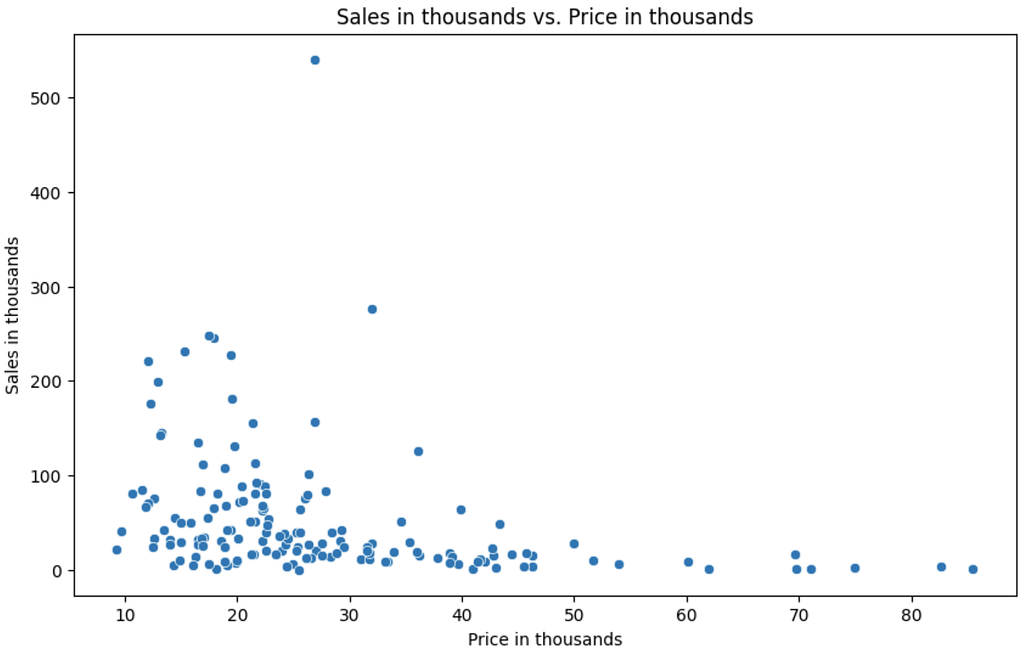
# Scatter plot of 'Sales in thousands' vs. 'Price in thousands'
plt.figure(figsize=(10, 6))
sns.scatterplot(x='Price in thousands', y='Sales in thousands', data=df)
plt.title('Sales in thousands vs. Price in thousands')
plt.show()
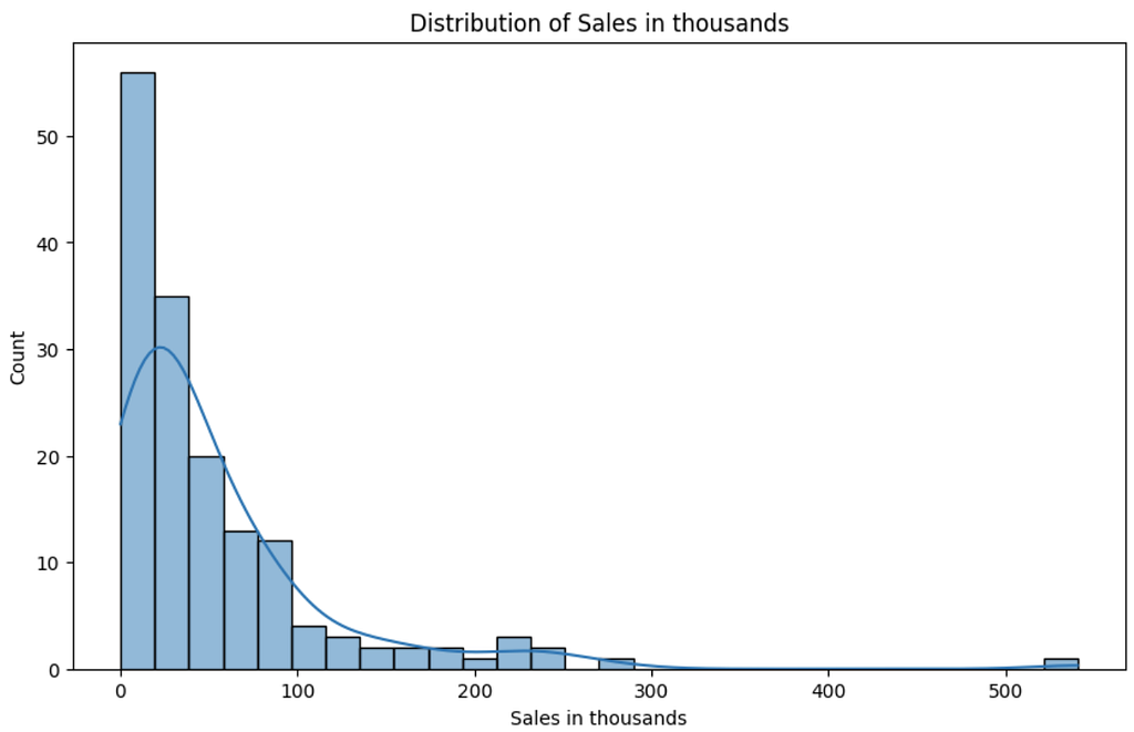
# Distribution of sale prices
plt.figure(figsize=(10, 6))
sns.histplot(df['Sales in thousands'], kde=True)
plt.title('Distribution of Sales in thousands')
plt.show()
Correlation Matrix of Numeric Features:
- This heatmap displays the correlation coefficients between the numeric features in the dataset. Strong positive or negative correlations are highlighted in deeper colors.
Scatter Plot of ‘Sales in thousands’ vs. ‘Price in thousands’:
- This scatter plot shows the relationship between the car sales (in thousands) and the price (in thousands).
Distribution of Sales in thousands:
- This histogram with a kernel density estimate (KDE) overlay shows the distribution of the car sales figures.
Grouping and Aggregation statistics:
Let’s continue with the analysis by performing grouping and aggregation on the car sales dataset. We’ll focus on calculating average sale prices by manufacturer, analyzing sales by year, and identifying the top 10 best-selling models.
import pandas as pd
import matplotlib.pyplot as plt
# Load the dataset
df = pd.read_csv("/mnt/data/Car_sales.csv")
# Convert columns to numeric types
numeric_columns = [
'4-year resale value', 'Price in thousands', 'Engine size',
'Horsepower', 'Wheelbase', 'Width', 'Length', 'Curb weight',
'Fuel capacity', 'Fuel efficiency'
]
for col in numeric_columns:
df[col] = pd.to_numeric(df[col], errors='coerce')
# Convert 'Latest Launch' to datetime type
df['Latest Launch'] = pd.to_datetime(df['Latest Launch'], errors='coerce')
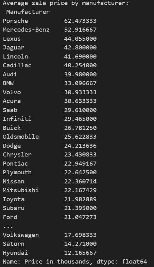
# Average sale price by manufacturer
avg_price_by_manufacturer = df.groupby('Manufacturer')['Price in thousands'].mean().sort_values(ascending=False)
print("Average sale price by manufacturer:\n", avg_price_by_manufacturer)
# Assuming Latest Launch represents the purchase date, extracting year from it
df['Year'] = df['Latest Launch'].dt.year
sales_by_year = df.groupby('Year')['Sales in thousands'].sum()
plt.figure(figsize=(12, 6))
sales_by_year.plot(kind='bar')
plt.title('Total Sales by Year')
plt.xlabel('Year')
plt.ylabel('Total Sales (in thousands)')
plt.show()
# Top 10 best-selling models
top_models = df['Model'].value_counts().head(10)
plt.figure(figsize=(12, 6))
top_models.plot(kind='bar')
plt.title('Top 10 Best-Selling Models')
plt.xlabel('Model')
plt.ylabel('Number of Sales')
plt.xticks(rotation=45, ha='right')
plt.tight_layout()
plt.show()
Calculate average sale price by manufacturer:
- Group the data by the ‘Manufacturer’ column.
- Compute the mean of ‘Price in thousands’ for each manufacturer.
- Sort the results in descending order of average price.
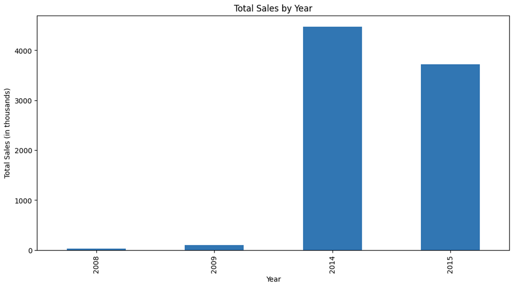
Analyze sales by year:
- Extract the year from the ‘Latest Launch’ column to create a new ‘Year’ column.
- Group the data by this ‘Year’ column.
- Sum the ‘Sales in thousands’ for each year.
- Plot the total sales by year using a bar chart.
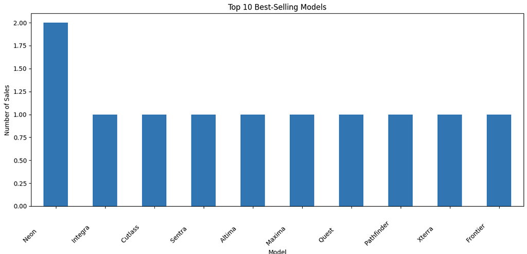
Identified the top 10 best-selling models:
- Count the occurrences of each model in the ‘Model’ column.
- Select the top 10 models based on the number of sales.
- Plot the top 10 best-selling models using a bar chart.
These steps help in understanding the average sale prices across different manufacturers, analyzing trends in sales over the years, and identifying the most popular car models.
- 5 Things I Wish I Knew Earlier in Python! 🐍
- 10 Essential Python Exercises
- Master Python’s Enumerate for Efficient Coding
Basic Statistical Measures
In this section, we’ll explore fundamental statistical measures that provide insights into our Car Sales dataset. We’ll cover measures of central tendency, dispersion, and distribution shape. These statistics will help us understand the typical values, variability, and overall characteristics of our data.
Measures of Central Tendency
We’ll calculate the mean, median, and mode for key numeric variables.
- Mean: The average value of each numeric column.
- Median: The middle value of each numeric column when sorted.
- Mode: The most frequent value of each numeric column.
# Measures of Central Tendency
mean_values = df[numeric_columns].mean()
median_values = df[numeric_columns].median()
mode_values = df[numeric_columns].mode().iloc[0]

print("Mean values:\n", mean_values)
print("\nMedian values:\n", median_values)
print("\nMode values:\n", mode_values)
Measures of Dispersion
We’ll calculate measures that describe the spread of our data, such as variance, standard deviation, and range.
- Variance: Measure of the spread of the data points from the mean.
- Standard Deviation: Square root of the variance, representing the average distance from the mean.
- Range: Difference between the maximum and minimum values.
# Measures of Dispersion
variance_values = df[numeric_columns].var()
std_dev_values = df[numeric_columns].std()
range_values = df[numeric_columns].max() - df[numeric_columns].min()

print("\nVariance values:\n", variance_values)
print("\nStandard Deviation values:\n", std_dev_values)
print("\nRange values:\n", range_values)
Measures of Distribution Shape
We’ll examine skewness and kurtosis to understand the shape of our distributions.
- Skewness: Measure of the asymmetry of the distribution.
- Kurtosis: Measure of the “tailedness” of the distribution.
# Measures of Distribution Shape
skewness_values = df[numeric_columns].skew()
kurtosis_values = df[numeric_columns].kurtosis()

print("\nSkewness values:\n", skewness_values)
print("\nKurtosis values:\n", kurtosis_values)
Percentiles and Quartiles
We’ll calculate key percentiles, including the 25th, 50th (median), and 75th percentiles.
- Percentiles: Values below which a certain percentage of data falls. Typically, the 25th, 50th, and 75th percentiles are calculated (first quartile, median, third quartile).
# Percentiles and Quartiles
percentiles = df[numeric_columns].quantile([0.25, 0.5, 0.75])
print("\nPercentiles:\n", percentiles)
Confidence Intervals
We’ll calculate a confidence interval for the mean sale price.
- Confidence Interval for Mean Sale Price: Range within which the true mean sale price is expected to fall, with a certain level of confidence (e.g., 95%).
from scipy import stats

# Confidence Intervals for mean sale price
sale_price_mean = df['Price in thousands'].mean()
sale_price_std = df['Price in thousands'].std()
confidence_level = 0.95
degrees_freedom = df['Price in thousands'].count() - 1
confidence_interval = stats.t.interval(confidence_level, degrees_freedom, sale_price_mean, sale_price_std/np.sqrt(df['Price in thousands'].count()))

print("\nConfidence interval for mean sale price:\n", confidence_interval)
Conclusion
This comprehensive guide has provided you with the foundational tools and techniques to perform statistical analysis using Python. By setting up a proper environment and leveraging powerful libraries like pandas, numpy, matplotlib, and seaborn, you can efficiently manipulate data, calculate essential statistical measures, and visualize your findings.
Understanding measures of central tendency, dispersion, and distribution shape, along with percentiles and confidence intervals, allows you to gain deep insights into your datasets.
Armed with these skills, you are now equipped to tackle real-world data challenges, uncovering hidden patterns and making informed decisions that can significantly impact your projects and career in software development or data science.
I believe I’ve left you in good hands. Now, it’s up to YOU to take this knowledge and go on to do your own data analysis, visualizations, and more.
Feel free to build on this code. Happy analyzing!
Unleash the Erase Powers in SQL
Interested in diving deeper into SQL and Database management? Discover a wealth of knowledge in my collection of articles on Medium, where I explore essential concepts, advanced techniques, and practical tips to enhance your skills.
Creating and Managing MySQL Tables

Final Words
Thank you for taking the time to read my article!
This article was first published on medium by CyCoderX.
Hey there! I’m CyCoderX, a data engineer who loves crafting end-to-end solutions. I write articles about Python, SQL, AI, Data Engineering, lifestyle and more! Join me as we explore the exciting world of tech, data, and beyond.
Interested in more content?
- For Python content and tips, click here to check out my list on Medium.
- For SQL, Databases, and data engineering content, click here to find out more!
Connect with me on social media:
- Medium: CyCoderX — Explore similar articles and updates.
- LinkedIn: CyCoderX — Connect with me professionally.
If you enjoyed this article, consider following me for future updates.
Please consider supporting me by:
- Clapping 50 times for this story
- Leaving a comment telling me your thoughts
- Highlighting your favorite part of the story
Car Sales Insights: Python Data Analysis Guide was originally published in Level Up Coding on Medium, where people are continuing the conversation by highlighting and responding to this story.
This content originally appeared on Level Up Coding - Medium and was authored by CyCoderX
CyCoderX | Sciencx (2024-07-09T16:43:08+00:00) Car Sales Insights: Python Data Analysis Guide. Retrieved from https://www.scien.cx/2024/07/09/car-sales-insights-python-data-analysis-guide/
Please log in to upload a file.
There are no updates yet.
Click the Upload button above to add an update.