This content originally appeared on Level Up Coding - Medium and was authored by Senthil E

Everything You Need to Know About GPU Programming with Python
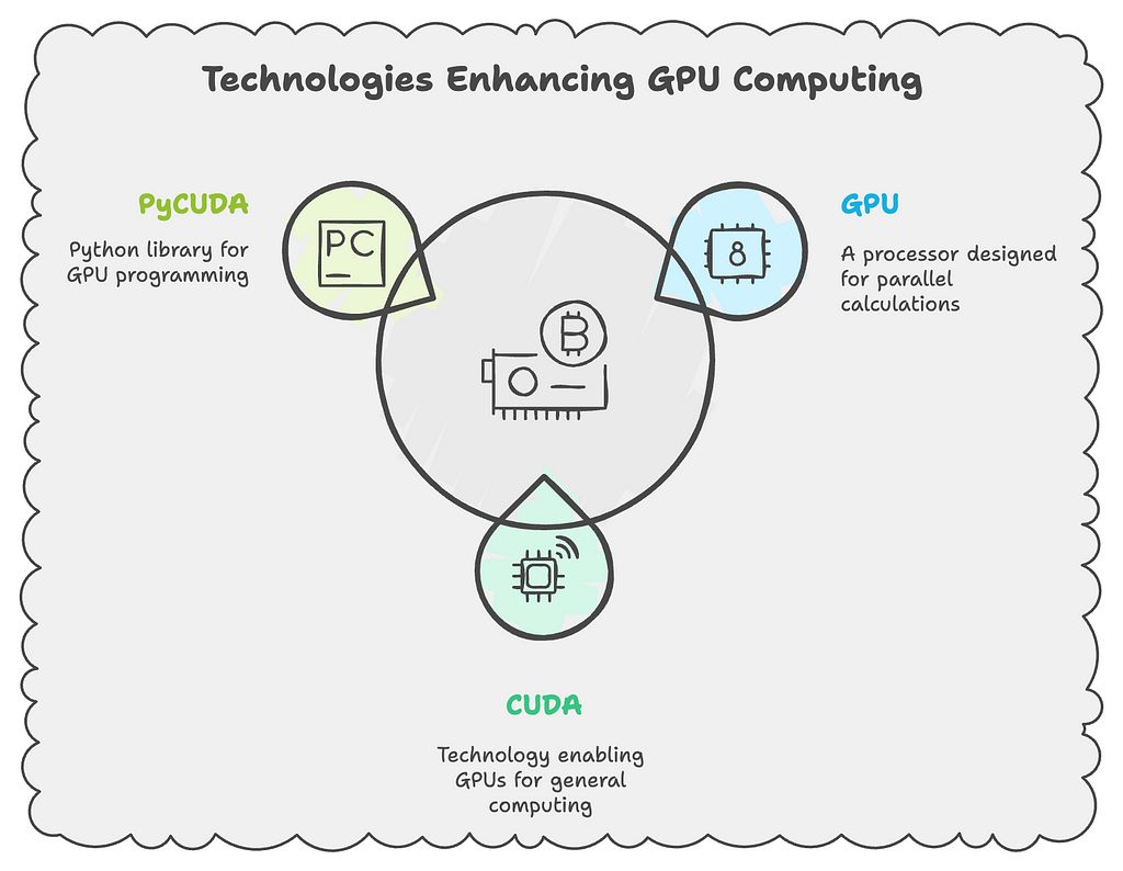
Introduction: The Evolution of GPU Computing
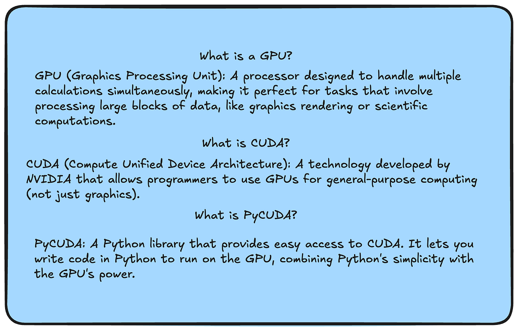
In 2006, NVIDIA revolutionized the computing landscape by introducing CUDA (Compute Unified Device Architecture), marking a pivotal moment in parallel computing history. While Graphics Processing Units (GPUs) were initially designed for rendering graphics and gaming, NVIDIA recognized their potential for general-purpose computing. This insight led to the development of CUDA, transforming GPUs from specialized graphics processors into powerful general-purpose computing engines.
Historical Context
The journey began in the early 2000s when researchers started experimenting with GPUs for non-graphical calculations, a concept known as GPGPU (General-Purpose Computing on Graphics Processing Units). However, this early work was challenging as programmers had to express their computational problems in terms of graphics operations using OpenGL or DirectX.
CUDA’s introduction in 2006 changed this paradigm completely. It provided developers with a more straightforward way to program GPUs using a C-like interface, eliminating the need to understand graphics programming. The first CUDA-capable GPU, the GeForce 8800 GTX, featured 128 parallel processor cores and demonstrated unprecedented computational capabilities for its time.

Technical Evolution
The CUDA architecture has evolved significantly since its inception:
- 2006 (G80): First unified graphics and computing GPU architecture
- 2008 (GT200): Introduction of double-precision floating-point operations
- 2010 (Fermi): First complete GPU computing architecture with L1/L2 caches
- 2012 (Kepler): Dynamic parallelism and Hyper-Q features
- 2014 (Maxwell): Improved memory hierarchy and power efficiency
- 2016 (Pascal): Unified memory and NVLink interconnect
- 2018 (Volta): Tensor Cores for AI acceleration
- 2020 (Ampere): Third-generation Tensor Cores and Multi-Instance GPU
- 2022 (Hopper): Fourth-generation Tensor Cores and Transformer Engine
Why CUDA Matters
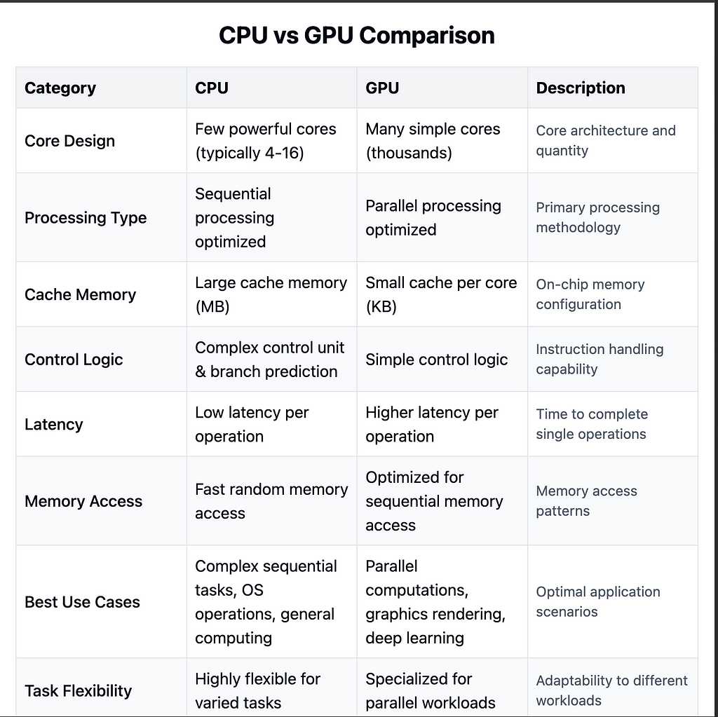
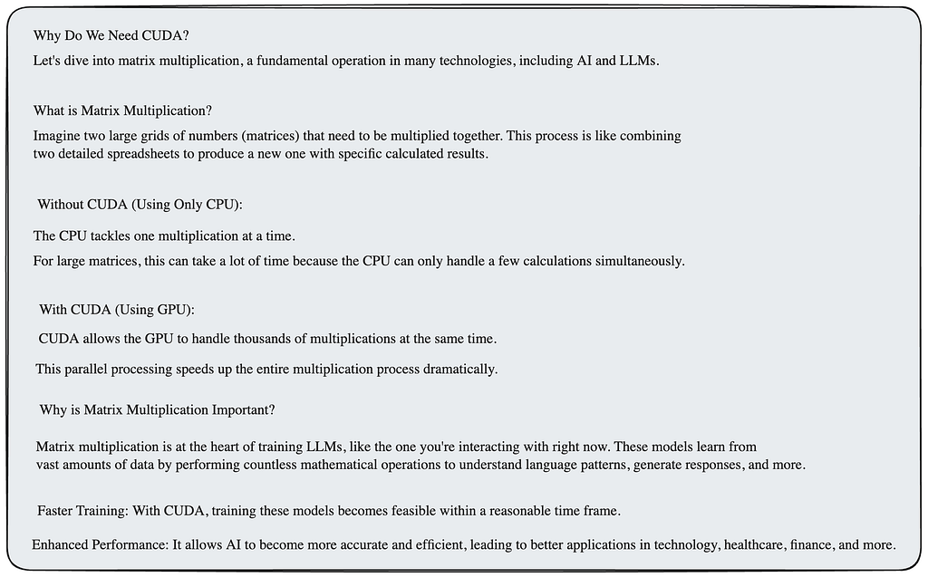
CUDA’s importance stems from its ability to harness the massive parallel processing power of GPUs. Modern GPUs contain thousands of small, efficient cores designed for handling multiple tasks simultaneously. For comparison:
- A typical CPU might have 8–32 cores
- NVIDIA’s A100 GPU features 6912 CUDA cores
- The latest H100 GPU contains 18,432 CUDA cores
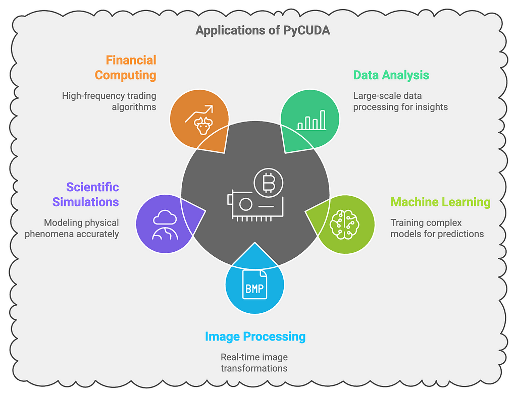
This parallel architecture makes GPUs exceptionally efficient for:
1. Deep Learning and AI computations
2. Scientific simulations
3. Cryptography
4. Image and video processing
5. Financial modeling
6. Molecular dynamics
7. Weather forecasting
Enter PyCUDA
While CUDA C/C++ provides low-level access to GPU computing, many developers prefer working with higher-level languages like Python. PyCUDA, developed by Andreas Klöckner in 2009, bridges this gap by providing Python bindings for CUDA. It enables developers to:
- Write GPU code using Python’s familiar syntax
- Maintain the performance benefits of CUDA
- Automatically manage GPU resources
- Integrate with popular Python scientific computing libraries
PyCUDA’s advantages include:
- Automatic memory management
- Runtime code generation
- Seamless integration with NumPy
- Error checking and debugging capabilities
- Object-oriented interface to CUDA operations
Modern GPU Architecture
Modern NVIDIA GPUs, like the A100 and H100, represent the pinnacle of GPU computing with features such as:
A100 (Ampere Architecture):
- 80GB HBM2e memory
- 1.6TB/s memory bandwidth
- 312 TFLOPS for AI training
- Multi-Instance GPU technology
- Third-generation Tensor Cores
H100 (Hopper Architecture):
- 80GB HBM3 memory
- 3TB/s memory bandwidth
- 1000 TFLOPS for AI training
- Fourth-generation Tensor Cores
- Transformer Engine for accelerated AI

Industry Impact
CUDA and GPU computing have transformed numerous industries:
- AI/ML: Enabled the deep learning revolution
- Healthcare: Accelerated medical image processing and drug discovery
- Finance: Enhanced real-time risk analysis and trading algorithms
- Scientific Research: Accelerated complex simulations
- Cloud Computing: Powered GPU-as-a-Service offerings
Before diving into PyCUDA programming, it’s crucial to understand why GPUs are fundamentally different from CPUs and how these differences enable massively parallel processing capabilities.
If you want to listen to this article, you need to sign into Google to listen to this podcast. The link is below
GPU vs CPU:
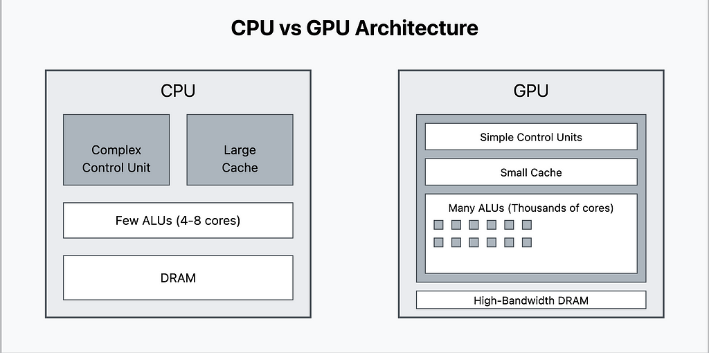
Understanding the Architecture Diagram:
CPU Architecture (Left Side):
1. Control Unit: — Large, sophisticated control logic — Complex branch prediction — Out-of-order execution — Advanced instruction pipelining
2. Cache Memory: — Large L1, L2, and L3 caches — Complex cache coherency protocols — Optimized for data reuse
3. Processing Units: — Few but powerful cores (typically 4–32) — Complex Arithmetic Logic Units (ALUs) — High clock speeds — Advanced vector processing units
GPU Architecture (Right Side):
- Control Unit: — Simplified control logic — Optimized for throughput — SIMD (Single Instruction, Multiple Data) focused
2. Cache Memory: — Small, fast cache per Streaming Multiprocessor (SM) — Optimized for throughput over latency — High-bandwidth memory interface
3. Processing Units: — Thousands of simple cores — Streamlined ALUs — Optimized for parallel operations — Specialized tensor cores for ML operations
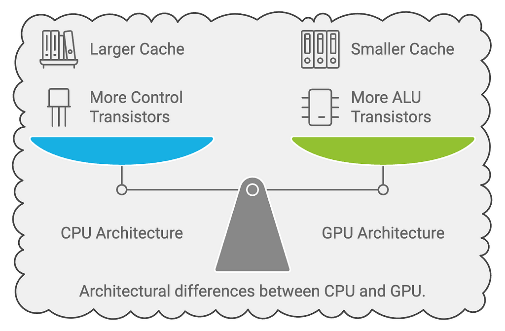
Processing Paradigms:
The architectural differences lead to fundamentally different approaches to handling computational tasks.
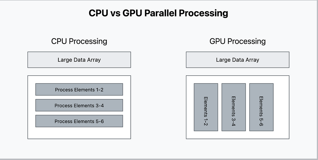
Understanding the Processing Diagram
CPU Processing Model (Left Side):
1. Sequential Execution:
— Tasks processed one after another
— Complex tasks handled efficiently
— High per-thread performance
— Optimized for serial workloads
2. Resource Utilization:
— Deep instruction pipelines
— Sophisticated task scheduling
— Dynamic resource allocation
GPU Processing Model (Right Side):
1. Parallel Execution:
— Many tasks processed simultaneously
— Simple tasks replicated across cores
— High aggregate throughput
— Optimized for parallel workloads
2. Resource Utilization:
— Wide SIMD execution
— Massive thread parallelism
— Hardware-managed scheduling
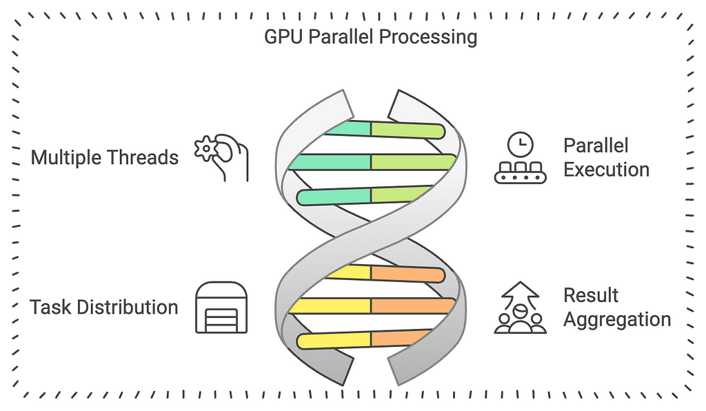
Real-World Impact
These architectural differences translate directly to performance characteristics:
CPU Excels At:
- Complex decision-making tasks
- Single-threaded applications
- Tasks with unpredictable branching
- Low-latency operations
- Operating system tasks
GPU Excels At:
- Parallel computations
- Matrix operations
- Image/video processing
- Deep learning training
- Scientific simulations
Memory Architecture and Bandwidth
Another crucial difference lies in memory architecture:
CPU Memory System:
- Standard DDR memory
- ~100 GB/s bandwidth
- Large memory capacity
- Complex cache hierarchy
GPU Memory System:
- High-bandwidth memory (HBM)
- ~1–3 TB/s bandwidth (A100/H100)
- Optimized for parallel access
- Specialized for compute workloads
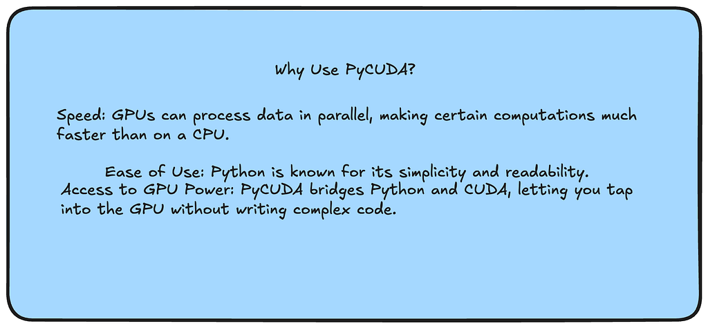
Setting Up Your Environment for PyCUDA
Before diving into PyCUDA programming, let’s ensure your system is properly configured. This section will guide you through the essential requirements and installation steps.
Prerequisites
1. NVIDIA GPU Requirements
First, verify that your system has a CUDA-capable NVIDIA GPU.
Minimum Requirements:
- NVIDIA GPU with Compute Capability 3.0 or higher
- At least 4GB GPU memory (recommended)
- Up-to-date NVIDIA drivers
To check your GPU:
import subprocess
def get_gpu_info():
 try:
    output = subprocess.check_output(
     ["nvidia-smi"],
     universal_newlines=True
     )
    print("GPU Information:")
    print(output)
 except:
    print("No NVIDIA GPU detected or nvidia-smi not installed")

get_gpu_info()
2. CUDA Toolkit Installation
CUDA Toolkit is essential for GPU programming. Follow these steps:
- Download CUDA Toolkit:
- Visit NVIDIA CUDA Downloads
- Select your operating system and version
- Follow the installation instructions
2. Verify Installation:
# Check CUDA version
nvcc --version
The expected output should show something like this:
3. Python Environment Setup
It’s recommended to use a virtual environment:
# Create a new virtual environment
python -m venv pycuda_env
# Activate the environment
# On Windows:
pycuda_env\Scripts\activate
# On Linux/Mac:
source pycuda_env/bin/activate
# Install required packages
pip install numpy
4. PyCUDA Installation
Install PyCUDA using pip:
pip install pycuda
5. Verifying Your Setup
Let’s verify everything is working with a simple PyCUDA program:
import pycuda.autoinit
import pycuda.driver as drv
import numpy as np
def verify_pycuda_setup():
    try:
        # Get device properties
        print(f"CUDA version: {drv.get_version()}")
        print(f"Device name: {pycuda.autoinit.device.name()}")
        print(f"Compute capability: {pycuda.autoinit.device.compute_capability()}")
        print(f"Total memory: {pycuda.autoinit.device.total_memory() // (1024*1024)} MB")

        # Try a simple operation
        a = np.random.randn(100).astype(np.float32)
        a_gpu = drv.mem_alloc(a.nbytes)
        drv.memcpy_htod(a_gpu, a)

        print("\nSuccessfully allocated and copied memory to GPU!")
        print("PyCUDA is working correctly!")

    except Exception as e:
        print(f"An error occurred: {str(e)}")
        print("Please check your installation.")
if __name__ == "__main__":
    verify_pycuda_setup()
Expected output (varies based on your GPU):
CUDA version: (11, 5, 0)
Device name: NVIDIA A100-SXM4-80GB
Compute capability: (8, 0)
Total memory: 81037 MB

Successfully allocated and copied memory to GPU!
PyCUDA is working correctly!

Understanding Basic PyCUDA Concepts
Before writing your first PyCUDA program, it’s essential to understand the fundamental concepts that form the foundation of GPU programming.
Key Terms and Concepts
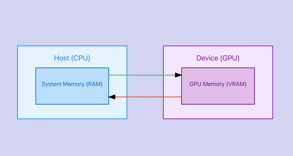
1. Host vs Device
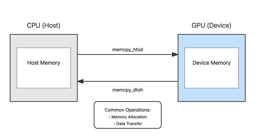
In GPU programming, we use specific terminology to distinguish between CPU and GPU:
- Host: Refers to the CPU and its memory (system RAM)
- Device: Refers to the GPU and its memory (VRAM)
2. Kernel Functions
A kernel is a special function that runs on the GPU. Key characteristics:
- Executes in parallel across many GPU threads
- Marked with `__global__` in CUDA C
- Called using special syntax with <<<>>> in PyCUDA
- Runs on the device (GPU)
Example of a simple kernel:
import pycuda.autoinit
import pycuda.driver as cuda
import numpy as np
from pycuda.compiler import SourceModule

# Define kernel with print statements
mod = SourceModule("""
#include <stdio.h>

__global__ void multiply_by_two(float *array)
{
    int idx = threadIdx.x + blockIdx.x * blockDim.x;

    // Print the index and value before multiplication
    printf("Before: idx = %d, value = %f\\n", idx, array[idx]);

    array[idx] *= 2;

    // Print the index and value after multiplication
    printf("After: idx = %d, value = %f\\n", idx, array[idx]);
}
""")

# Get function from module
multiply_by_two = mod.get_function("multiply_by_two")

# Create a sample array
array_size = 10
array = np.random.randn(array_size).astype(np.float32)

# Print original array in Python
print("Original array:")
print(array)

# Allocate memory on the device and copy array to device
array_gpu = cuda.mem_alloc(array.nbytes)
cuda.memcpy_htod(array_gpu, array)

# Execute the kernel with one block of 10 threads
multiply_by_two(array_gpu, block=(array_size, 1, 1), grid=(1, 1))

# Copy the result back from the device
cuda.memcpy_dtoh(array, array_gpu)

# Print the modified array in Python
print("\nModified array (after multiply_by_two):")
print(array)
Original array:
[-4.3534854e-01  7.7988309e-01  6.1468828e-01 -1.5304610e-03
  1.1495910e+00  7.5472385e-01  2.4845517e+00  8.3205029e-02
  7.3480928e-01 -1.6091207e-01]

Modified array (after multiply_by_two):
[-8.7069708e-01  1.5597662e+00  1.2293766e+00 -3.0609220e-03
  2.2991819e+00  1.5094477e+00  4.9691033e+00  1.6641006e-01
  1.4696186e+00 -3.2182413e-01]
Before: idx = 0, value = -0.435349
Before: idx = 1, value = 0.779883
Before: idx = 2, value = 0.614688
Before: idx = 3, value = -0.001530
Before: idx = 4, value = 1.149591
Before: idx = 5, value = 0.754724
Before: idx = 6, value = 2.484552
Before: idx = 7, value = 0.083205
Before: idx = 8, value = 0.734809
Before: idx = 9, value = -0.160912
After: idx = 0, value = -0.870697
After: idx = 1, value = 1.559766
After: idx = 2, value = 1.229377
After: idx = 3, value = -0.003061
After: idx = 4, value = 2.299182
After: idx = 5, value = 1.509448
After: idx = 6, value = 4.969103
After: idx = 7, value = 0.166410
After: idx = 8, value = 1.469619
After: idx = 9, value = -0.321824
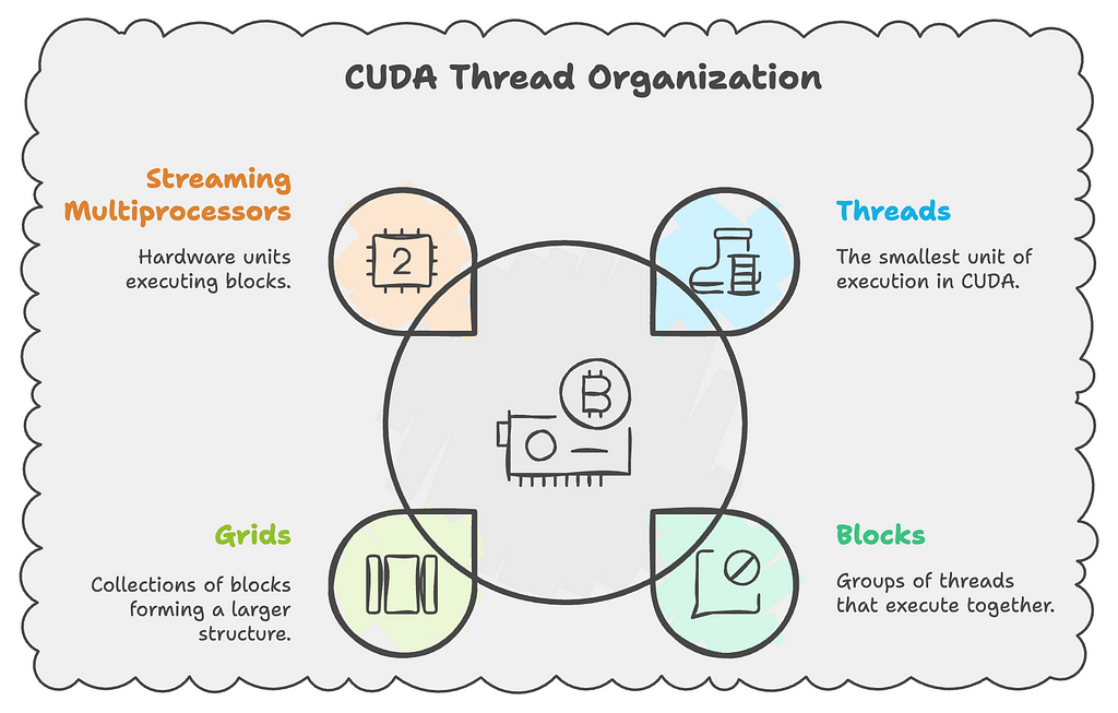
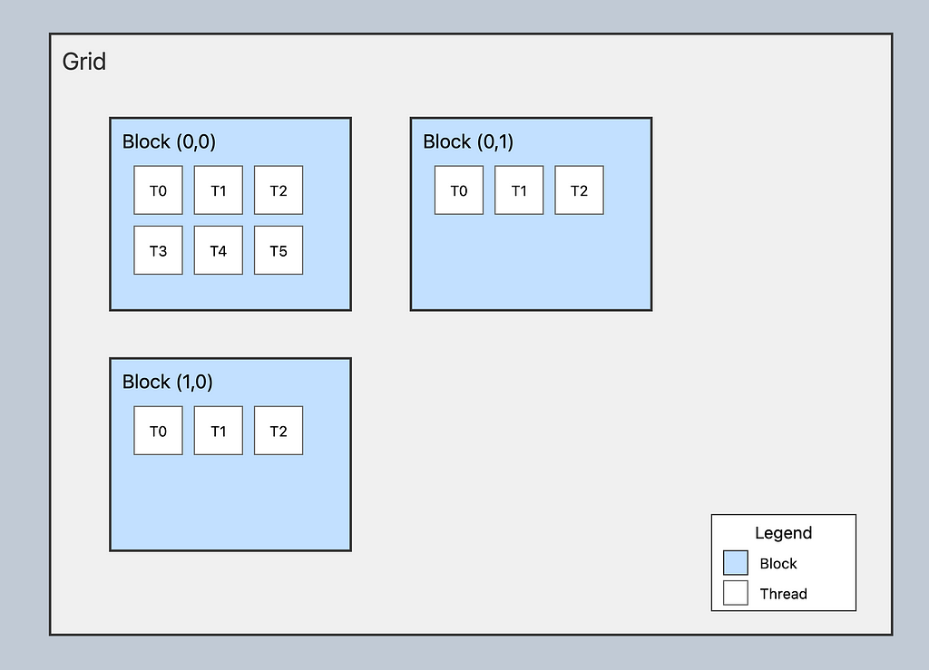
3. Threads and Blocks
GPU programming uses a hierarchical threading model:
- Threads:
- Smallest unit of execution
- Each thread runs the kernel function
- Has unique coordinates (threadIdx.x, threadIdx.y, threadIdx.z)
2. Blocks:
- Group of threads that can cooperate
- Share memory resources
- Has coordinates (blockIdx.x, blockIdx.y, blockIdx.z)
3. Grid:
- Collection of blocks
- Organized in 1D, 2D, or 3D
Deep Dive: Understanding CUDA Execution Hierarchy
Let’s break down these concepts using simple analogies to make them clearer:
1. Kernel
- Think of it as a special function that runs on the GPU
- Like a recipe that many cooks follow simultaneously
- Each kernel runs the same code but on different data
- In PyCUDA, this is your CUDA C code wrapped in SourceModule
2. Thread
- The smallest unit of execution in CUDA
- Like a single worker executing the kernel code
- Each thread works on its own piece of data
- Can think of it as one instance of your kernel running
3. Warp
- A group of 32 threads that execute together
- All threads in a warp execute the same instruction at the same time
- Like a team of 32 workers moving in perfect sync
- Hardware-level grouping (you can’t change the size)
4. Block
- A programmable group of threads (up to 1024 threads)
- Threads in a block can communicate and share memory
- Like a department of workers in the same room
- Multiple warps make up a block
5. Grid
- Collection of blocks
- Like multiple departments working on the same project
- Blocks in a grid can’t directly communicate
- The entire GPU program is organized as a grid

Restaurant Kitchen Analogy
To better understand how these concepts work together, think of a large restaurant kitchen:
1. Kernel is like a recipe (e.g., “cut vegetables”)
2. Thread is like a single cook following that recipe
3. Warp is like a team of 32 cooks working in perfect sync
4. Block is like a kitchen station with multiple teams
5. Grid is like the entire kitchen with multiple stations
Key Points for Beginners
- All threads in a warp execute the same instruction at the same time
- Threads within a block can share resources (shared memory)
- Blocks are independent and can execute in any order
- The GPU automatically manages the execution of warps
- When you write kernel code, you write it from a single thread’s perspective
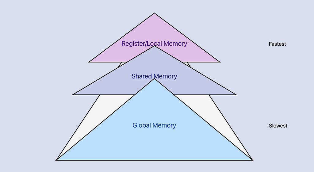
4. Memory Types
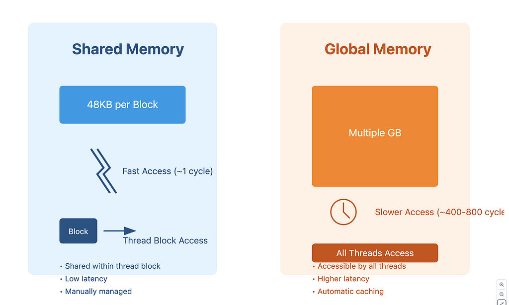
CUDA provides different types of memory:
1. Global Memory:
— Accessible by all threads
— Largest but slowest
— Main way to transfer data between host and device
2. Shared Memory:
— Shared between threads in a block
— Much faster than global memory
— Limited size (usually around 48KB per block)
3. Local Memory:
— Private to each thread
— Automatically managed
— Used for thread-local variables
4. Constant Memory:
— Read-only
— Cached for fast access
— Accessible by all threads
5. Basic Data Transfer
Moving data between host and device involves three main steps:
- Allocation:
# Allocate memory on GPU
import pycuda.driver as drv
gpu_array = drv.mem_alloc(cpu_array.nbytes)
2. Transfer:
# Host to Device (H2D)
drv.memcpy_htod(gpu_array, cpu_array)
# Device to Host (D2H)
drv.memcpy_dtoh(cpu_array, gpu_array)
3. Deallocation:
# Free GPU memory
gpu_array.free()
Understanding Memory Flow
Here’s a complete example showing memory transfer:
import pycuda.autoinit
import pycuda.driver as drv
import numpy as np

# Create data on CPU
cpu_data = np.random.randn(1000).astype(np.float32)

# Allocate GPU memory
gpu_data = drv.mem_alloc(cpu_data.nbytes)

# Transfer to GPU
drv.memcpy_htod(gpu_data, cpu_data)

# Transfer back to CPU
result = np.empty_like(cpu_data)
drv.memcpy_dtoh(result, gpu_data)

# Verify
print("Data transfer successful:", np.allclose(cpu_data, result))
Data transfer successful: True
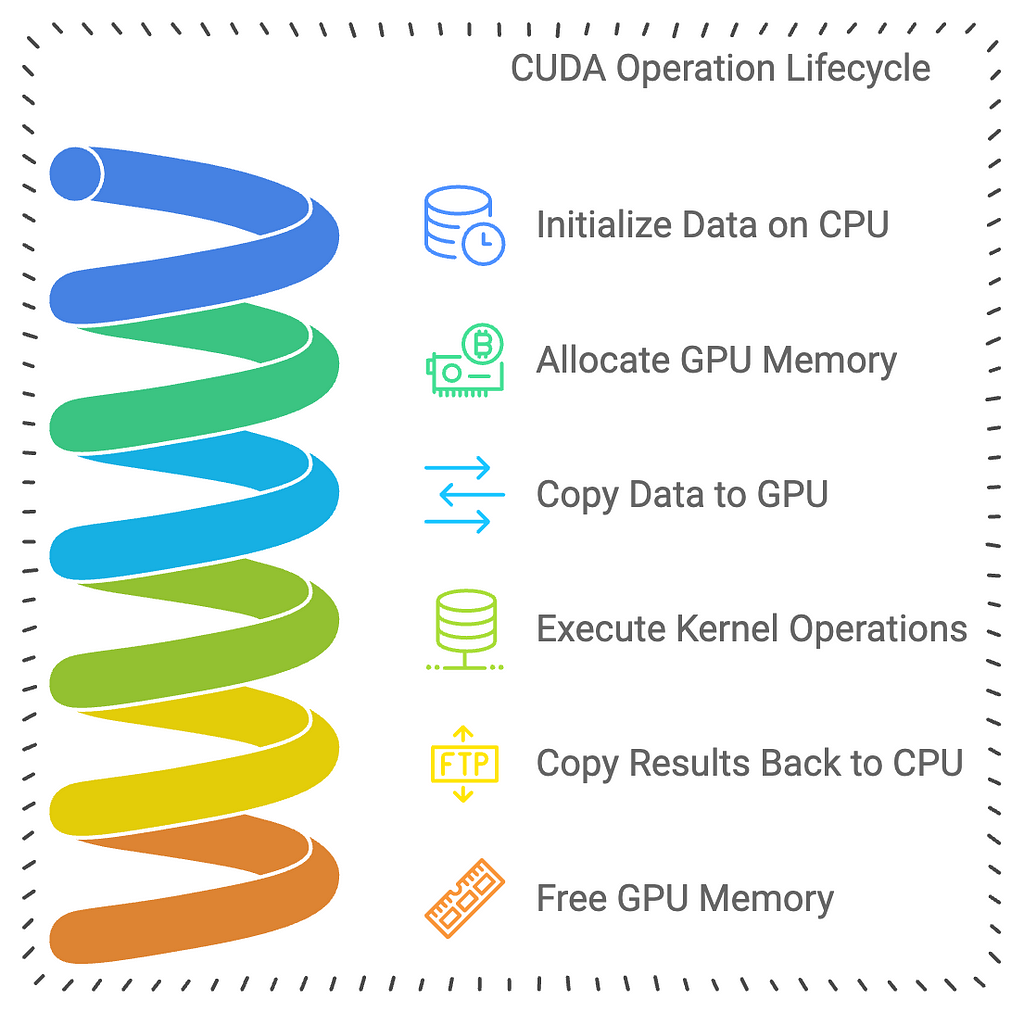
Your First PyCUDA Program
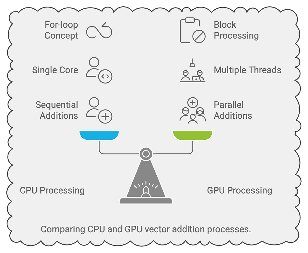
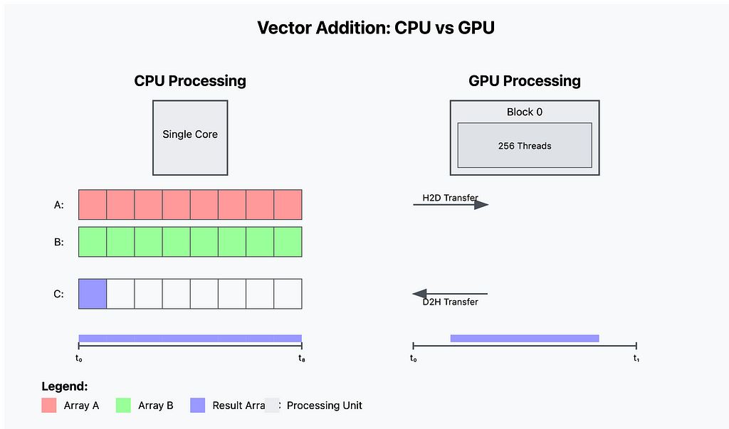
Let’s create a simple yet comprehensive example of vector addition that demonstrates the basic workflow of GPU programming. We’ll add two vectors element by element, breaking down each step and discussing important concepts along the way.
Vector Addition Example
Step 1: Basic Setup and Imports
import pycuda.autoinit
import pycuda.driver as drv
import numpy as np
from pycuda.compiler import SourceModule
Step 2: Writing the CUDA Kernel
# Define the kernel in CUDA C
cuda_kernel = """
__global__ void vector_add(float *a, float *b, float *result, int n)
{
    // Calculate unique thread index
    int idx = threadIdx.x + blockIdx.x * blockDim.x;

    // Check if thread is within array bounds
    if (idx < n)
    {
        result[idx] = a[idx] + b[idx];
    }
}
"""
# Compile the kernel
mod = SourceModule(cuda_kernel)
# Get a reference to the kernel function
vector_add = mod.get_function("vector_add")
Step 3: Preparing the Data
def prepare_data(n):
    # Create input vectors
    a = np.random.randn(n).astype(np.float32)
    b = np.random.randn(n).astype(np.float32)

    # Create output vector
    result = np.zeros_like(a)

    return a, b, result
Step 4: Configuring Grid and Block Dimensions
def calculate_grid_block_size(n):
    # Maximum threads per block for most GPUs
    max_threads_per_block = 512

    # Calculate block size
    block_size = min(max_threads_per_block, n)

    # Calculate grid size
    grid_size = (n + block_size - 1) // block_size

    return (grid_size, 1, 1), (block_size, 1, 1)
Step 5: Complete Vector Addition Program
def gpu_vector_add(a, b, n):
    # Calculate grid and block dimensions
    grid_dim, block_dim = calculate_grid_block_size(n)

    # Allocate output array
    result = np.zeros_like(a)

    # Call the kernel
    vector_add(
        # Inputs
        drv.In(a), drv.In(b), drv.Out(result), np.int32(n),
        # Grid and block dimensions
        grid=grid_dim, block=block_dim
    )

    return result
# Example usage
def main():
    # Vector size
    n = 1_000_000

    # Prepare data
    a, b, expected_result = prepare_data(n)

    # Perform GPU computation
    result = gpu_vector_add(a, b, n)

    # Verify results
    print("Correct result:", np.allclose(result, a + b))
Code Breakdown
- Kernel Function (vector_add):
- Takes input arrays (a, b), output array (result), and size (n)
- Calculates unique thread index
- Performs addition only if index is within bounds
- Each thread handles one element of the arrays
2. Thread Index Calculation:
- threadIdx.x: Position within the block
- blockIdx.x: Block number
- blockDim.x: Block size
- Formula: idx = threadIdx.x + blockIdx.x * blockDim.x
3.Memory Management:
- drv.In: Copies data from host to device
- drv.Out: Allocates device memory and copies result back
- Automatic cleanup when function returns
Common Pitfalls
- Array Type Mismatch
# Wrong: Mixed types
a = np.random.randn(1000)  # defaults to float64
# Fix: Explicitly use float32
a = np.random.randn(1000).astype(np.float32)
2. Index Out of Bounds
# Wrong: No bounds checking
if (idx < n)  # Missing this check
    result[idx] = a[idx] + b[idx];  # Potential memory error
3. Block Size Too Large
# Wrong: Exceeding maximum threads per block
block_dim = (2000, 1, 1)  # Too large
# Fix: Use calculate_grid_block_size function
4. Memory Leaks
# Wrong: Manual memory allocation without freeing
gpu_array = drv.mem_alloc(a.nbytes)
# Better: Use drv.In and drv.Out for automatic management
Best Practices
- Data Types
- Always use np.float32 instead of np.float64
- Convert data types explicitly
- Check data type consistency
2. Error Handling
try:
    result = gpu_vector_add(a, b, n)
except Exception as e:
    print(f"GPU operation failed: {e}")
3. Performance Optimization
- Use power of 2 for block sizes when possible
- Align memory access patterns
- Balance block size and grid size
4.Memory Management
- Use automatic memory management when possible
- Clear GPU memory after large operations
- Monitor GPU memory usage
5. Validation
def validate_inputs(a, b):
    assert a.dtype == np.float32, "Array must be float32"
    assert a.shape == b.shape, "Arrays must have same shape"
    assert a.flags.c_contiguous, "Array must be contiguous"
Adding Two Lists Together
We’ll start by adding two lists of numbers using regular Python code (runs on the CPU) and then show how to do the same using PyCUDA (runs on the GPU).
Adding Lists on the CPU
# Create two lists of numbers
a = [1, 2, 3, 4, 5]
b = [10, 20, 30, 40, 50]
# Create an empty list to store the results
c = []
# Loop through the lists and add corresponding elements
for i in range(len(a)):
    c.append(a[i] + b[i])
# Display the result
print("Sum:", c)
Explanation:
- We have two lists a and b.
- We loop through each element, add them, and store the result in list c.
- The CPU processes each addition one after another.
Output:
Sum: [11, 22, 33, 44, 55]
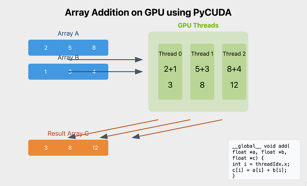
Adding Lists on the GPU with PyCUDA
Now, let’s perform the same operation using PyCUDA to utilize the GPU’s power.
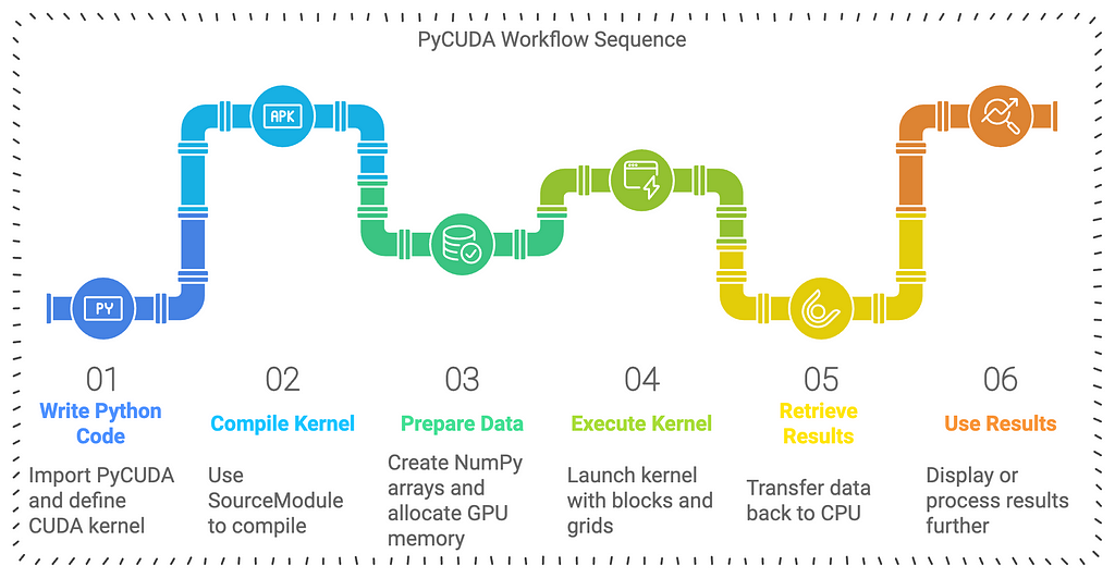
Step 1: Install PyCUDA
Ensure PyCUDA is installed on your system.
pip install pycuda
Note: You need an NVIDIA GPU and CUDA Toolkit installed for PyCUDA to work.
Step 2: Import Necessary Libraries
import pycuda.autoinit  # Initializes the CUDA driver
import pycuda.driver as cuda  # Access to CUDA functionalities
import numpy as np  # Library for efficient array computations
from pycuda.compiler import SourceModule  # Compiles CUDA code
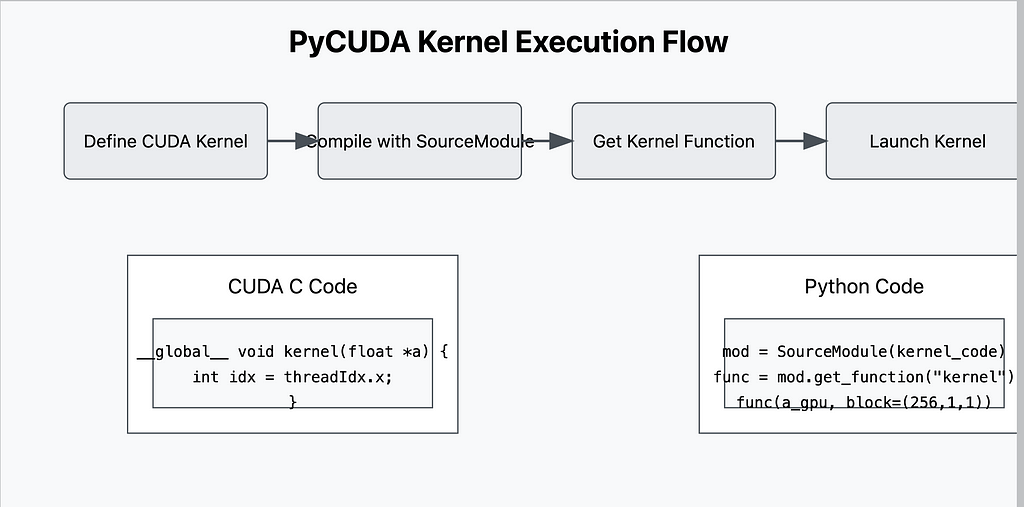
Step 3: Write the GPU Function (Kernel)
kernel_code = """
__global__ void add_arrays(float *a, float *b, float *c)
{
    int idx = threadIdx.x;  // Unique index for each thread
    c[idx] = a[idx] + b[idx];  // Perform addition
}
"""
Explanation:
- __global__: Indicates that the function runs on the GPU and can be called from the CPU.
- float *a, *b, *c: These are pointers to arrays of floating-point numbers.
- int idx = threadIdx.x;: Each thread (worker) gets a unique index.
- c[idx] = a[idx] + b[idx];: Each thread adds one pair of numbers.
Step 4: Compile the Kernel
mod = SourceModule(kernel_code)  # Compiles the kernel code
add_arrays = mod.get_function("add_arrays")  # Gets the compiled function
Step 5: Prepare the Data
# Create NumPy arrays (they work well with PyCUDA)
a = np.array([1, 2, 3, 4, 5], dtype=np.float32)
b = np.array([10, 20, 30, 40, 50], dtype=np.float32)
c = np.empty_like(a)  # Empty array to store the result
Explanation:
- We use np.array to create arrays that are compatible with PyCUDA.
- dtype=np.float32 ensures the data type matches what the GPU expects.
- np.empty_like(a) creates an empty array with the same shape and type as a.
Step 6: Run the Kernel
# Number of threads (one per element)
threads_per_block = len(a)
# Execute the kernel function
add_arrays(
    cuda.In(a), cuda.In(b), cuda.Out(c),  # Input and output arrays
    block=(threads_per_block, 1, 1),  # Define the block size
    grid=(1, 1)  # Define the grid size
)
Explanation:
- cuda.In(a) and cuda.In(b): Transfers input arrays to the GPU.
- cuda.Out(c): Prepares to receive the output array from the GPU.
- block=(threads_per_block, 1, 1): Sets up the number of threads in a block.
- grid=(1, 1): Number of blocks; we use one block here.
Step 7: Display the Results
print("Array a:", a)
print("Array b:", b)
print("Sum c:", c)
Output:
Array a: [1. 2. 3. 4. 5.]
Array b: [10. 20. 30. 40. 50.]
Sum c: [11. 22. 33. 44. 55.]
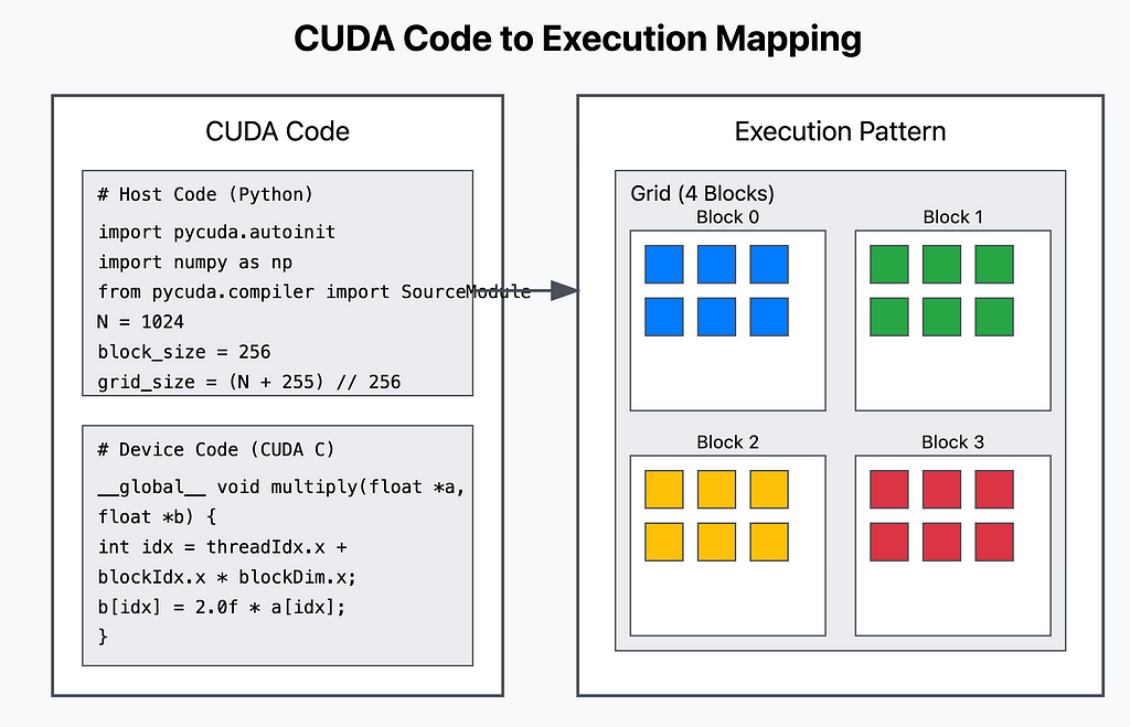
Understanding How the GPU Executes the Code
- Parallel Execution: The GPU runs multiple threads simultaneously. Each thread handles the addition for one pair of numbers.
- Threads and Blocks: We defined a block with as many threads as there are elements in the array.
- Indexing with threadIdx.x: Each thread uses its unique index to operate on the correct elements.
Simplifying the Concepts
- Thread: Think of a thread as a worker assigned to a specific task.
- Kernel Function: Instructions that each worker (thread) follows.
- Block: A group of workers that can share resources.
- Grid: A collection of blocks, organizing the workers for large tasks.
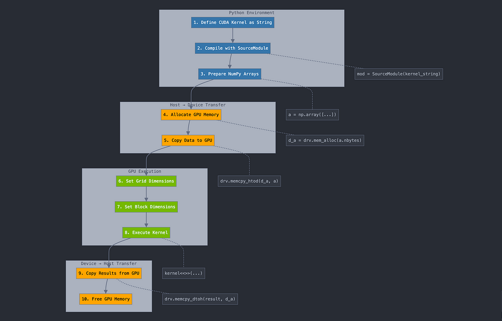
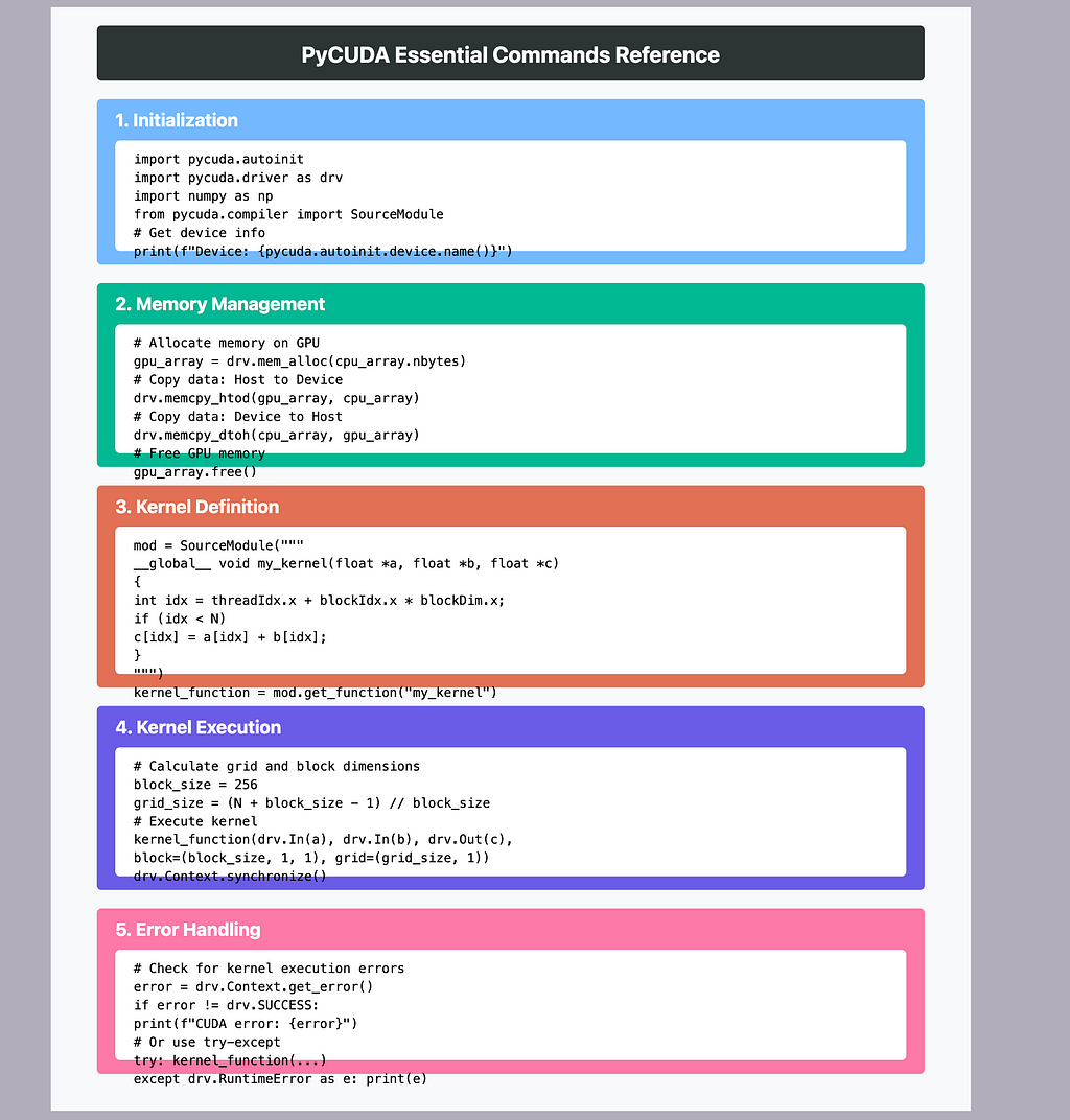
Essential PyCUDA Operations:
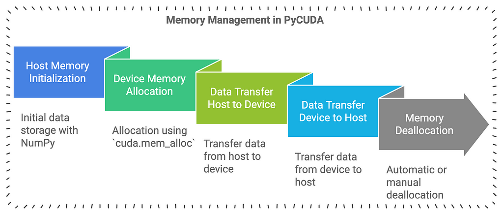
- Memory Management
a) Allocation:
import pycuda.autoinit
import pycuda.driver as drv
import numpy as np
# Host array creation
host_array = np.random.rand(1000).astype(np.float32)
# GPU memory allocation methods:
# Method 1: Using cuda.mem_alloc
gpu_array = drv.mem_alloc(host_array.nbytes)
# Method 2: Using gpuarray
from pycuda import gpuarray
gpu_array = gpuarray.to_gpu(host_array)
b) Transfer:
# Host to Device transfer
drv.memcpy_htod(gpu_array, host_array)
# Device to Host transfer
result_host = np.empty_like(host_array)
drv.memcpy_dtoh(result_host, gpu_array)
c) Deallocation:
# Free GPU memory
gpu_array.free()
# Or if using gpuarray:
del gpu_array
- Array Operations
a) Vector Addition Example:
from pycuda.compiler import SourceModule
mod = SourceModule("""
__global__ void add_vectors(float *a, float *b, float *c, int n)
{
    int idx = threadIdx.x + blockIdx.x * blockDim.x;
    if (idx < n)
        c[idx] = a[idx] + b[idx];
}
""")
# Get function from module
add_vectors = mod.get_function("add_vectors")
# Prepare data
n = 1000000
a = np.random.randn(n).astype(np.float32)
b = np.random.randn(n).astype(np.float32)
c = np.zeros_like(a)
# Execute kernel
add_vectors(
    drv.In(a), drv.In(b), drv.Out(c), np.int32(n),
    block=(256, 1, 1), grid=((n + 255) // 256, 1)
)
- Error Handling
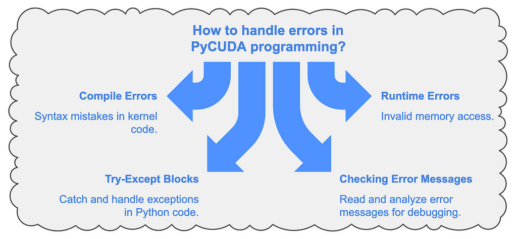
a) Basic Error Checking:
# After kernel execution
cuda_error = drv.Context.synchronize()
if cuda_error:
    raise RuntimeError(f"CUDA error: {cuda_error}")
# Or using explicit error checking
error = drv.Context.get_error()
if error != drv.Success:
    raise RuntimeError(f"CUDA error: {error}")
b) Memory Error Prevention:
try:
    # Get device properties
    device = drv.Device(0)
    max_threads = device.get_attribute(drv.device_attribute.MAX_THREADS_PER_BLOCK)
    max_grid_dim = device.get_attribute(drv.device_attribute.MAX_GRID_DIMENSIONS)

    # Use these limits when launching kernels
    block_size = min(256, max_threads)
    grid_size = (n + block_size - 1) // block_size

except drv.RuntimeError as e:
    print(f"CUDA Error: {e}")
Best Practices:
- Memory Management:
- Always free GPU memory after use
- Use asynchronous transfers for better performance when possible
- Minimize host-device transfers
2. Kernel Optimization:
- Choose appropriate block sizes (usually multiples of 32)
- Consider memory coalescing for better performance
- Use shared memory for frequently accessed data
3. Error Handling:
- Always check for CUDA errors after kernel launches
- Implement proper error handling for memory operations
- Use compute-sanitizer for debugging memory issues

Thread and Block Management in CUDA programming
1. Thread Structure and Basic Concepts:
import pycuda.autoinit
import pycuda.driver as drv
from pycuda.compiler import SourceModule
# Basic kernel showing thread structure
kernel_code = """
__global__ void thread_example(int *output) {
    // Thread identification
    int tid = threadIdx.x;                     // Thread ID within block
    int bid = blockIdx.x;                      // Block ID
    int bdim = blockDim.x;                     // Block dimension
    int gid = threadIdx.x + blockIdx.x * blockDim.x;  // Global thread ID

    // Store thread info
    output[gid] = gid;
}
"""
mod = SourceModule(kernel_code)
thread_example = mod.get_function("thread_example")
2.Block Organization Example:
# Example of 2D block organization
kernel_2d = """
__global__ void matrix_operation(float *matrix, int width, int height) {
    // 2D Thread and Block indexing
    int row = blockIdx.y * blockDim.y + threadIdx.y;
    int col = blockIdx.x * blockDim.x + threadIdx.x;

    if (row < height && col < width) {
        int idx = row * width + col;
        matrix[idx] = row + col;  // Example operation
    }
}
"""
mod = SourceModule(kernel_2d)
matrix_operation = mod.get_function("matrix_operation")
# Example usage
width, height = 1024, 1024
matrix = np.zeros((height, width), dtype=np.float32)
# Define block and grid dimensions
block_dim = (16, 16, 1)  # 16x16 threads per block
grid_dim = ((width + block_dim[0] - 1) // block_dim[0],
            (height + block_dim[1] - 1) // block_dim[1],
            1)
matrix_operation(
    drv.Out(matrix), np.int32(width), np.int32(height),
    block=block_dim, grid=grid_dim
)
3. Grid Configuration Example:
# Function to calculate optimal grid and block dimensions
def calculate_grid_block_dim(total_elements, max_threads_per_block=1024):
    """
    Calculate optimal grid and block dimensions
    """
    # Get device properties
    device = drv.Device(0)
    max_threads = device.get_attribute(drv.device_attribute.MAX_THREADS_PER_BLOCK)
    max_block_dim = min(max_threads_per_block, max_threads)

    # Calculate dimensions
    block_dim = min(total_elements, max_block_dim)
    grid_dim = (total_elements + block_dim - 1) // block_dim

    return grid_dim, block_dim

# Example usage
n = 1000000
grid_dim, block_dim = calculate_grid_block_dim(n)
print(f"Grid size: {grid_dim}, Block size: {block_dim}")
4. Optimizing Thread/Block Dimensions:
kernel_optimization = """
__global__ void optimized_operation(float *input, float *output, int n) {
    // Shared memory for block-level data
    __shared__ float shared_data[256];

    int tid = threadIdx.x;
    int gid = blockIdx.x * blockDim.x + threadIdx.x;

    // Load data into shared memory
    if (gid < n) {
        shared_data[tid] = input[gid];
    }
    __syncthreads();  // Ensure all threads have loaded data

    // Process data using shared memory
    if (gid < n) {
        output[gid] = shared_data[tid] * 2.0f;  // Example operation
    }
}
"""
Important Concepts:
- Thread Identification:
- threadIdx: Thread index within a block (x, y, z)
- blockIdx: Block index within the grid (x, y, z)
- blockDim: Dimensions of block (threads per block)
- gridDim: Dimensions of grid (blocks per grid)
2. Memory Considerations:
- Shared memory is shared between threads in a block
- Global memory is accessible by all threads
- Local memory is private to each thread
3. Optimization Guidelines:
- Use power of 2 for block dimensions
- Consider hardware limits (max threads per block)
- Balance between block size and number of blocks
- Consider memory coalescing for better performance
4. Common Pitfalls:
- Exceeding maximum thread/block limits
- Insufficient blocks for good occupancy
- Not checking array bounds
- Not synchronizing threads when necessary
Example of calculating optimal dimensions for a 2D matrix:
def get_optimal_block_dims(width, height):
    max_threads = 1024  # Typical maximum threads per block

    # Start with 16x16 block size (common for 2D operations)
    block_x = min(16, width)
    block_y = min(16, height)

    # Calculate grid dimensions
    grid_x = (width + block_x - 1) // block_x
    grid_y = (height + block_y - 1) // block_y

    return (grid_x, grid_y), (block_x, block_y)
# Example usage
width, height = 2048, 1024
grid_dim, block_dim = get_optimal_block_dims(width, height)
print(f"Grid dimensions: {grid_dim}")
print(f"Block dimensions: {block_dim}")
Common Pycuda Patterns
import pycuda.autoinit
import pycuda.driver as drv
import numpy as np
from pycuda.compiler import SourceModule

# 1. Map Operation Example - Square each element
map_kernel = SourceModule("""
__global__ void square_elements(float *a, int n)
{
    int idx = threadIdx.x + blockIdx.x * blockDim.x;
    if (idx < n)
        a[idx] = a[idx] * a[idx];
}
""")

def demonstrate_map():
    # Create input data
    n = 10
    a = np.random.randn(n).astype(np.float32)
    a_copy = a.copy()  # Keep a copy for verification

    # Get the kernel function
    square = map_kernel.get_function("square_elements")

    # Allocate memory and copy data to GPU
    a_gpu = drv.mem_alloc(a.nbytes)
    drv.memcpy_htod(a_gpu, a)

    # Execute kernel
    square(a_gpu, np.int32(n), block=(256, 1, 1), grid=((n + 255) // 256, 1))

    # Get results back
    drv.memcpy_dtoh(a, a_gpu)

    print("\nMap Operation (Squaring Elements):")
    print("Input:", a_copy)
    print("Output:", a)
    print("Verification (CPU):", a_copy ** 2)

# 2. Reduce Operation Example - Sum all elements
reduce_kernel = SourceModule("""
__global__ void reduce_sum(float *a, float *out, int n)
{
    __shared__ float sdata[256];
    unsigned int tid = threadIdx.x;
    unsigned int i = blockIdx.x * blockDim.x + threadIdx.x;

    sdata[tid] = (i < n) ? a[i] : 0;
    __syncthreads();

    for (unsigned int s = blockDim.x / 2; s > 0; s >>= 1) {
        if (tid < s) {
            sdata[tid] += sdata[tid + s];
        }
        __syncthreads();
    }

    if (tid == 0) out[blockIdx.x] = sdata[0];
}
""")

def demonstrate_reduce():
    # Create input data
    n = 1000
    a = np.random.randn(n).astype(np.float32)

    # Get the kernel function
    reduce = reduce_kernel.get_function("reduce_sum")

    # Calculate number of blocks needed
    num_blocks = (n + 255) // 256
    out = np.zeros(num_blocks, dtype=np.float32)

    # Execute kernel
    reduce(drv.In(a), drv.Out(out), np.int32(n),
           block=(256, 1, 1), grid=(num_blocks, 1))

    print("\nReduce Operation (Sum):")
    print("Input array size:", n)
    print("GPU sum:", np.sum(out))
    print("CPU sum:", np.sum(a))
    print("Difference:", abs(np.sum(out) - np.sum(a)))

# 3. Scan Operation Example - Cumulative sum
scan_kernel = SourceModule("""
__global__ void scan(float *input, float *output, int n)
{
    __shared__ float temp[256];
    int thid = threadIdx.x;

    int offset = 1;
    temp[thid] = input[thid];
    __syncthreads();

    for (int d = n>>1; d > 0; d >>= 1)
    {
        if (thid < d)
        {
            int ai = offset*(2*thid+1)-1;
            int bi = offset*(2*thid+2)-1;
            temp[bi] += temp[ai];
        }
        offset *= 2;
        __syncthreads();
    }

    output[thid] = temp[thid];
}
""")

def demonstrate_scan():
    # Create input data
    n = 8  # Using small size for demonstration
    a = np.random.randn(n).astype(np.float32)

    # Get the kernel function
    scan = scan_kernel.get_function("scan")

    # Execute kernel
    out = np.zeros_like(a)
    scan(drv.In(a), drv.Out(out), np.int32(n),
         block=(n, 1, 1), grid=(1, 1))

    print("\nScan Operation (Cumulative Sum):")
    print("Input:", a)
    print("GPU scan:", out)
    print("CPU scan (verification):", np.cumsum(a))

# 4. Element-wise Operation Example - Vector addition
elementwise_kernel = SourceModule("""
__global__ void vector_add(float *a, float *b, float *c, int n)
{
    int idx = threadIdx.x + blockIdx.x * blockDim.x;
    if (idx < n)
        c[idx] = a[idx] + b[idx];
}
""")

def demonstrate_elementwise():
    # Create input data
    n = 10
    a = np.random.randn(n).astype(np.float32)
    b = np.random.randn(n).astype(np.float32)

    # Get the kernel function
    vector_add = elementwise_kernel.get_function("vector_add")

    # Execute kernel
    c = np.zeros_like(a)
    vector_add(drv.In(a), drv.In(b), drv.Out(c), np.int32(n),
              block=(256, 1, 1), grid=((n + 255) // 256, 1))

    print("\nElement-wise Operation (Vector Addition):")
    print("Vector A:", a)
    print("Vector B:", b)
    print("GPU Result (A + B):", c)
    print("CPU Result (verification):", a + b)

# Run all demonstrations
if __name__ == "__main__":
    demonstrate_map()
    demonstrate_reduce()
    demonstrate_scan()
    demonstrate_elementwise()
Map Operation (Squaring Elements):
Input: [-1.0795693  -0.49946883 -0.85547155 -0.11256783 -1.809529   -2.3715997
  0.7603225  -0.8601724  -0.5761283  -0.47840685]
Output: [1.16547    0.24946912 0.73183155 0.01267152 3.274395   5.624485
 0.5780903  0.73989654 0.3319238  0.2288731 ]
Verification (CPU): [1.16547    0.24946912 0.73183155 0.01267152 3.274395   5.624485
 0.5780903  0.73989654 0.3319238  0.2288731 ]

Reduce Operation (Sum):
Input array size: 1000
GPU sum: -6.51562
CPU sum: -6.515627
Difference: 6.67572e-06

Scan Operation (Cumulative Sum):
Input: [-0.88912827  1.2799991  -0.06190103  0.66699725 -0.28361192  0.39906275
  1.0735904  -0.22892074]
GPU scan: [-0.88912827  0.39087087 -0.06190103  0.9959671  -0.28361192  0.11545083
  1.0735904   1.9560876 ]
CPU scan (verification): [-0.88912827  0.39087087  0.32896984  0.9959671   0.71235514  1.1114179
  2.1850083   1.9560876 ]

Element-wise Operation (Vector Addition):
Vector A: [-0.38900524 -0.5881734  -1.8390615  -1.0052649   0.19294897 -0.62156844
  0.29566982  0.8197685  -0.5074794   0.23306295]
Vector B: [-0.11977915 -1.2113439  -0.25459185  0.11812047  0.9040481  -0.07971474
  0.8966112  -0.5862821  -0.4948726   0.82815486]
GPU Result (A + B): [-0.5087844  -1.7995173  -2.0936534  -0.8871444   1.096997   -0.70128316
  1.192281    0.23348641 -1.002352    1.0612178 ]
CPU Result (verification): [-0.5087844  -1.7995173  -2.0936534  -0.8871444   1.096997   -0.70128316
  1.192281    0.23348641 -1.002352    1.0612178 ]
- Map Operation: This is the simplest pattern where we apply the same operation to each element independently. In our example, we square each element of an array.
Input:  [1, 2, 3, 4]
         ↓  ↓  ↓  ↓    (square each element)
Output: [1, 4, 9, 16]
2. Reduce Operation: This pattern combines all elements into a single result. In our example, we sum all elements in parallel using a tree-based approach.
Level 0:  [1  2  3  4  5  6  7  8]
Level 1:  [3     7     11    15  ]
Level 2:  [10         26        ]
Level 3:  [36                   ]
3. Scan Operation: This pattern computes running totals. Each output element contains the sum of all previous input elements.
Input:  [1  2  3  4  5]
Output: [1  3  6  10 15]
        ↑  ↑  ↑   ↑   ↑
        1  1+2  1+2+3  etc.
4. Element-wise Operation: This pattern performs operations between corresponding elements of multiple arrays. In our example, we add two vectors element by element.
Array A: [1  2  3  4]
Array B: [5  6  7  8]
         ↓  ↓  ↓  ↓    (add corresponding elements)
Output: [6  8  10 12]
Each pattern demonstrates different aspects of parallel processing:
- Map shows independent parallel operations
- Reduce shows parallel aggregation
- Scan shows parallel prefix sums
- Element-wise shows parallel operations between multiple arrays
The key advantage of using GPU for these patterns is that operations can be performed on many elements simultaneously, rather than one at a time as would be done on a CPU.
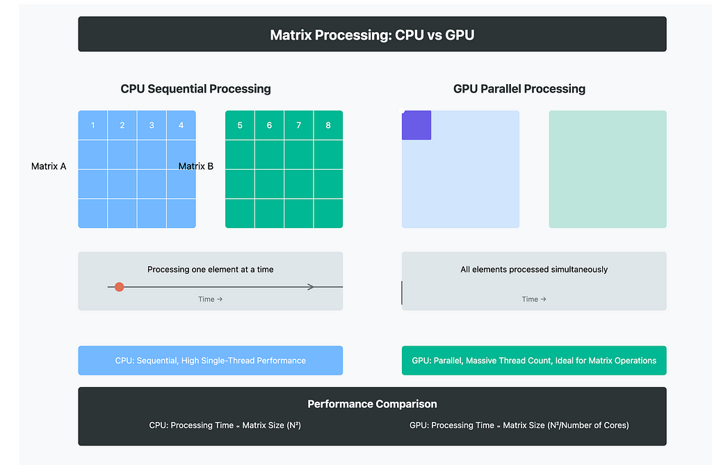
Practical PyCUDA examples with real-world applications
import pycuda.autoinit
import pycuda.driver as drv
import numpy as np
from pycuda.compiler import SourceModule

# 1. Image Processing Examples

# 1.1 RGB to Grayscale Conversion
rgb_to_gray_kernel = SourceModule("""
__global__ void rgb_to_grayscale(unsigned char *rgb, unsigned char *gray, int width, int height)
{
    int x = threadIdx.x + blockIdx.x * blockDim.x;
    int y = threadIdx.y + blockIdx.y * blockDim.y;

    if (x < width && y < height) {
        int idx = y * width + x;
        int rgb_idx = idx * 3;
        // Standard grayscale conversion weights
        gray[idx] = (unsigned char)(
            0.299f * rgb[rgb_idx] +     // Red
            0.587f * rgb[rgb_idx + 1] + // Green
            0.114f * rgb[rgb_idx + 2]   // Blue
        );
    }
}
""")

def demonstrate_grayscale():
    # Create sample RGB image (100x100 pixels)
    width, height = 100, 100
    rgb_image = np.random.randint(0, 256, (height, width, 3), dtype=np.uint8)
    gray_image = np.zeros((height, width), dtype=np.uint8)

    # Get the kernel function
    rgb_to_gray = rgb_to_gray_kernel.get_function("rgb_to_grayscale")

    # Execute kernel with 16x16 thread blocks
    block_size = (16, 16, 1)
    grid_size = ((width + block_size[0] - 1) // block_size[0],
                 (height + block_size[1] - 1) // block_size[1])

    rgb_to_gray(
        drv.In(rgb_image), drv.Out(gray_image),
        np.int32(width), np.int32(height),
        block=block_size, grid=grid_size
    )

    print("\nGrayscale Conversion:")
    print("Original RGB shape:", rgb_image.shape)
    print("Grayscale shape:", gray_image.shape)
    print("Sample pixel (RGB):", rgb_image[0, 0])
    print("Sample pixel (Gray):", gray_image[0, 0])

# 1.2 Simple Blur Filter
blur_kernel = SourceModule("""
__global__ void blur_filter(unsigned char *input, unsigned char *output, int width, int height)
{
    int x = threadIdx.x + blockIdx.x * blockDim.x;
    int y = threadIdx.y + blockIdx.y * blockDim.y;

    if (x < width && y < height) {
        int idx = y * width + x;
        float sum = 0.0f;
        int count = 0;

        // Simple 3x3 average blur
        for(int dy = -1; dy <= 1; dy++) {
            for(int dx = -1; dx <= 1; dx++) {
                int nx = x + dx;
                int ny = y + dy;

                if(nx >= 0 && nx < width && ny >= 0 && ny < height) {
                    sum += input[ny * width + nx];
                    count++;
                }
            }
        }

        output[idx] = (unsigned char)(sum / count);
    }
}
""")

def demonstrate_blur():
    # Create sample grayscale image
    width, height = 100, 100
    input_image = np.random.randint(0, 256, (height, width), dtype=np.uint8)
    output_image = np.zeros_like(input_image)

    # Get the kernel function
    blur = blur_kernel.get_function("blur_filter")

    # Execute kernel
    block_size = (16, 16, 1)
    grid_size = ((width + block_size[0] - 1) // block_size[0],
                 (height + block_size[1] - 1) // block_size[1])

    blur(
        drv.In(input_image), drv.Out(output_image),
        np.int32(width), np.int32(height),
        block=block_size, grid=grid_size
    )

    print("\nBlur Filter:")
    print("Input shape:", input_image.shape)
    print("Sample 3x3 region before blur:\n", input_image[0:3, 0:3])
    print("Sample 3x3 region after blur:\n", output_image[0:3, 0:3])

# 2. Matrix Operations

# 2.1 Matrix Multiplication
matrix_mul_kernel = SourceModule("""
__global__ void matrix_multiply(float *a, float *b, float *c, int m, int n, int p)
{
    int row = threadIdx.y + blockIdx.y * blockDim.y;
    int col = threadIdx.x + blockIdx.x * blockDim.x;

    if (row < m && col < p) {
        float sum = 0;
        for (int k = 0; k < n; k++) {
            sum += a[row * n + k] * b[k * p + col];
        }
        c[row * p + col] = sum;
    }
}
""")

def demonstrate_matrix_multiply():
    # Create sample matrices
    m, n, p = 4, 3, 2  # Small matrices for demonstration
    a = np.random.randn(m, n).astype(np.float32)
    b = np.random.randn(n, p).astype(np.float32)
    c = np.zeros((m, p), dtype=np.float32)

    # Get the kernel function
    matrix_multiply = matrix_mul_kernel.get_function("matrix_multiply")

    # Execute kernel
    block_size = (16, 16, 1)
    grid_size = ((p + block_size[0] - 1) // block_size[0],
                 (m + block_size[1] - 1) // block_size[1])

    matrix_multiply(
        drv.In(a), drv.In(b), drv.Out(c),
        np.int32(m), np.int32(n), np.int32(p),
        block=block_size, grid=grid_size
    )

    print("\nMatrix Multiplication:")
    print("Matrix A:\n", a)
    print("Matrix B:\n", b)
    print("Result (GPU):\n", c)
    print("Result (CPU verification):\n", np.dot(a, b))

# 2.2 Matrix Transpose
transpose_kernel = SourceModule("""
__global__ void matrix_transpose(float *input, float *output, int width, int height)
{
    int x = threadIdx.x + blockIdx.x * blockDim.x;
    int y = threadIdx.y + blockIdx.y * blockDim.y;

    if (x < width && y < height) {
        output[x * height + y] = input[y * width + x];
    }
}
""")

def demonstrate_transpose():
    # Create sample matrix
    width, height = 4, 3
    input_matrix = np.random.randn(height, width).astype(np.float32)
    output_matrix = np.zeros((width, height), dtype=np.float32)

    # Get the kernel function
    transpose = transpose_kernel.get_function("matrix_transpose")

    # Execute kernel
    block_size = (16, 16, 1)
    grid_size = ((width + block_size[0] - 1) // block_size[0],
                 (height + block_size[1] - 1) // block_size[1])

    transpose(
        drv.In(input_matrix), drv.Out(output_matrix),
        np.int32(width), np.int32(height),
        block=block_size, grid=grid_size
    )

    print("\nMatrix Transpose:")
    print("Input matrix:\n", input_matrix)
    print("Transposed (GPU):\n", output_matrix)
    print("Transposed (CPU verification):\n", input_matrix.T)

# Run demonstrations
if __name__ == "__main__":
    demonstrate_grayscale()
    demonstrate_blur()
    demonstrate_matrix_multiply()
    demonstrate_transpose()
Grayscale Conversion:
Original RGB shape: (100, 100, 3)
Grayscale shape: (100, 100)
Sample pixel (RGB): [ 20 193 233]
Sample pixel (Gray): 145

Blur Filter:
Input shape: (100, 100)
Sample 3x3 region before blur:
 [[ 14 251  61]
 [136  80  77]
 [221 229   9]]
Sample 3x3 region after blur:
 [[120 103 144]
 [155 119 125]
 [149 113  73]]

Matrix Multiplication:
Matrix A:
 [[-0.66616106 -0.10933682  0.5089306 ]
 [-0.12389754 -0.28968918  0.97915065]
 [ 0.14836024  0.61603856 -0.20268178]
 [-0.74302     0.47540665 -0.32892975]]
Matrix B:
 [[-1.8884981   0.39611024]
 [ 2.1660886  -1.6947594 ]
 [ 0.52779263  1.1569128 ]]
Result (GPU):
 [[ 1.2898206   0.51021475]
 [ 0.12327631  1.5746683 ]
 [ 0.9472421  -1.2197553 ]
 [ 2.2593582  -1.4805607 ]]

Result (CPU verification):
 [[ 1.2898206   0.51021475]
 [ 0.12327631  1.5746683 ]
 [ 0.9472421  -1.2197553 ]
 [ 2.2593582  -1.4805607 ]]

Matrix Transpose:
Input matrix:
 [[ 0.92167944 -1.2641314  -0.10569248  0.9058027 ]
 [-0.5706148   0.74336165  2.5295794   0.15187392]
 [-0.06107518  0.76098543  0.71997863  0.93019915]]
Transposed (GPU):
 [[ 0.92167944 -0.5706148  -0.06107518]
 [-1.2641314   0.74336165  0.76098543]
 [-0.10569248  2.5295794   0.71997863]
 [ 0.9058027   0.15187392  0.93019915]]
Transposed (CPU verification):
 [[ 0.92167944 -0.5706148  -0.06107518]
 [-1.2641314   0.74336165  0.76098543]
 [-0.10569248  2.5295794   0.71997863]
 [ 0.9058027   0.15187392  0.93019915]]
A. RGB to Grayscale Conversion: This is a fundamental image processing operation that converts color images to black and white.
RGB Image (3 channels)     Grayscale Image (1 channel)
[R G B]                    [Gray]
[230 120 40]     →        [150]
The conversion uses weighted sums of RGB values:
- Gray = 0.299×Red + 0.587×Green + 0.114×Blue
2. Blur Filter: A simple 3x3 average blur that smooths the image by averaging each pixel with its neighbors.
Original Image     Blurred Image
[5 2 7]           [4 4 5]
[1 9 3]    →      [4 5 4]
[6 4 8]           [5 5 6]
3.Matrix Operations
A. Matrix Multiplication: Multiplies two matrices in parallel. Each thread computes one element of the result matrix.
Matrix A    Matrix B    Result C
[1 2]      [5 6]       [19 22]
[3 4]  ×   [7 8]   =   [43 50]
4. Matrix Transpose: Flips a matrix over its diagonal, turning rows into columns and vice versa.
Original Matrix    Transposed Matrix
[1 2 3]           [1 4]
[4 5 6]     →     [2 5]
                  [3 6]
The advantages of using GPU for these operations are:
- Image Processing:
- Each pixel can be processed independently
- Perfect for parallel processing
- Especially efficient for large images
2. Matrix Operations:
- Many calculations can be done simultaneously
- Significant speedup for large matrices
- Essential for deep learning applications
Basic CUDA performance optimization techniques:
import pycuda.autoinit
import pycuda.driver as drv
from pycuda.compiler import SourceModule
import numpy as np
import time

# 1. Thread Configuration Optimization
thread_config_kernel = SourceModule("""
__global__ void vector_add(float *a, float *b, float *c, int n)
{
    int idx = threadIdx.x + blockIdx.x * blockDim.x;
    if (idx < n)
        c[idx] = a[idx] + b[idx];
}
""")

def test_thread_configurations():
    # Test data
    n = 10000000
    a = np.random.randn(n).astype(np.float32)
    b = np.random.randn(n).astype(np.float32)
    c = np.zeros_like(a)

    vector_add = thread_config_kernel.get_function("vector_add")

    # Test different thread configurations
    thread_configs = [32, 64, 128, 256, 512, 1024]
    times = []

    print("\nThread Configuration Tests:")
    print("Threads per Block | Grid Size | Time (ms)")
    print("-" * 45)

    for threads_per_block in thread_configs:
        grid_size = (n + threads_per_block - 1) // threads_per_block

        # Time the kernel execution
        start = drv.Event()
        end = drv.Event()

        start.record()
        vector_add(
            drv.In(a), drv.In(b), drv.Out(c), np.int32(n),
            block=(threads_per_block, 1, 1), grid=(grid_size, 1)
        )
        end.record()
        end.synchronize()

        time_ms = start.time_till(end)
        times.append(time_ms)

        print(f"{threads_per_block:^15} | {grid_size:^9} | {time_ms:^8.2f}")

# 2. Memory Transfer Optimization
def demonstrate_memory_transfer():
    n = 10000000
    data = np.random.randn(n).astype(np.float32)

    print("\nMemory Transfer Tests:")

    # Test 1: Multiple small transfers
    start_time = time.time()
    chunk_size = 1000000
    for i in range(0, n, chunk_size):
        chunk = data[i:i+chunk_size]
        gpu_mem = drv.mem_alloc(chunk.nbytes)
        drv.memcpy_htod(gpu_mem, chunk)
    small_transfer_time = time.time() - start_time

    # Test 2: Single large transfer
    start_time = time.time()
    gpu_mem = drv.mem_alloc(data.nbytes)
    drv.memcpy_htod(gpu_mem, data)
    large_transfer_time = time.time() - start_time

    print(f"Multiple small transfers: {small_transfer_time:.4f} seconds")
    print(f"Single large transfer: {large_transfer_time:.4f} seconds")
    print(f"Speedup: {small_transfer_time/large_transfer_time:.2f}x")

# 3. Coalesced vs Non-coalesced Memory Access
coalesced_kernel = SourceModule("""
// Coalesced memory access
__global__ void coalesced_access(float *input, float *output, int n)
{
    int idx = threadIdx.x + blockIdx.x * blockDim.x;
    if (idx < n)
        output[idx] = input[idx];
}

// Non-coalesced memory access (strided)
__global__ void noncoalesced_access(float *input, float *output, int n)
{
    int idx = threadIdx.x + blockIdx.x * blockDim.x;
    if (idx < n/2)
        output[idx] = input[idx * 2];
}
""")

def demonstrate_memory_access():
    n = 10000000
    input_data = np.random.randn(n).astype(np.float32)
    output_data = np.zeros_like(input_data)

    coalesced = coalesced_kernel.get_function("coalesced_access")
    noncoalesced = coalesced_kernel.get_function("noncoalesced_access")

    print("\nMemory Access Pattern Tests:")

    # Test coalesced access
    start = drv.Event()
    end = drv.Event()
    start.record()

    coalesced(
        drv.In(input_data), drv.Out(output_data), np.int32(n),
        block=(256, 1, 1), grid=((n + 255) // 256, 1)
    )

    end.record()
    end.synchronize()
    coalesced_time = start.time_till(end)

    # Test non-coalesced access
    start.record()

    noncoalesced(
        drv.In(input_data), drv.Out(output_data), np.int32(n),
        block=(256, 1, 1), grid=((n + 255) // 256, 1)
    )

    end.record()
    end.synchronize()
    noncoalesced_time = start.time_till(end)

    print(f"Coalesced access time: {coalesced_time:.2f} ms")
    print(f"Non-coalesced access time: {noncoalesced_time:.2f} ms")
    print(f"Slowdown factor: {noncoalesced_time/coalesced_time:.2f}x")

# 4. Basic Profiling Example
def profile_kernel_execution():
    n = 10000000
    input_data = np.random.randn(n).astype(np.float32)

    # Create events for timing
    start = drv.Event()
    end = drv.Event()

    print("\nKernel Profiling:")
    print("Operation            | Time (ms)")
    print("-" * 35)

    # Time memory allocation
    start.record()
    gpu_mem = drv.mem_alloc(input_data.nbytes)
    end.record()
    end.synchronize()
    print(f"Memory allocation    | {start.time_till(end):8.2f}")

    # Time host to device transfer
    start.record()
    drv.memcpy_htod(gpu_mem, input_data)
    end.record()
    end.synchronize()
    print(f"Host to Device copy  | {start.time_till(end):8.2f}")

    # Time kernel execution
    square = thread_config_kernel.get_function("vector_add")
    start.record()
    square(gpu_mem, gpu_mem, gpu_mem, np.int32(n),
           block=(256, 1, 1), grid=((n + 255) // 256, 1))
    end.record()
    end.synchronize()
    print(f"Kernel execution     | {start.time_till(end):8.2f}")

    # Time device to host transfer
    start.record()
    drv.memcpy_dtoh(input_data, gpu_mem)
    end.record()
    end.synchronize()
    print(f"Device to Host copy  | {start.time_till(end):8.2f}")

if __name__ == "__main__":
    test_thread_configurations()
    demonstrate_memory_transfer()
    demonstrate_memory_access()
    profile_kernel_execution()
Thread Configuration Tests:
Threads per Block | Grid Size | Time (ms)
---------------------------------------------
      32        |  312500   |  26.43
      64        |  156250   |  29.92
      128       |   78125   |  29.33
      256       |   39063   |  29.32
      512       |   19532   |  29.35
     1024       |   9766    |  29.25

Memory Transfer Tests:
Multiple small transfers: 0.0124 seconds
Single large transfer: 0.0085 seconds
Speedup: 1.46x

Memory Access Pattern Tests:
Coalesced access time: 16.55 ms
Non-coalesced access time: 19.77 ms
Slowdown factor: 1.20x

Kernel Profiling:
Operation            | Time (ms)
-----------------------------------
Memory allocation    |     0.43
Host to Device copy  |     8.27
Kernel execution     |     0.17
Device to Host copy  |     6.47
- Thread Configuration Optimization
This involves finding the optimal number of threads per block. Key points:
- Too few threads: GPU underutilized
- Too many threads: resource constraints
- Sweet spot often between 128 and 512 threads
Threads/Block:  32   64   128   256   512   1024
Performance:    ▂    ▄    ▆    █     ▆     ▄
2. Memory Transfer Optimization
Demonstrates the importance of batch transfers:
- Small transfers: High overhead
- Large transfers: Better bandwidth utilization
Multiple small transfers:
[Data] → [GPU] → [Data] → [GPU] → [Data] → [GPU]
(Slow, high overhead)
Single large transfer:
[Data Data Data Data] → [GPU]
(Fast, low overhead)
3.Coalesced vs Non-coalesced Memory Access
Shows the importance of memory access patterns:
- Coalesced: Adjacent threads access adjacent memory
- Non-coalesced: Scattered memory access
Coalesced Access:
Thread 0: [0] →
Thread 1: [1] →  Memory: [0][1][2][3]
Thread 2: [2] →
Thread 3: [3] →
Non-coalesced Access:
Thread 0: [0] ----→
Thread 1: [2] ----→  Memory: [0][1][2][3]
Thread 2: [4] ----→
Thread 3: [6] ----→
4. Basic Profiling
Shows how to measure performance of different operations:
- Memory allocation
- Data transfer (H2D and D2H)
- Kernel execution
|--alloc--|--H2D--|--kernel--|--D2H--|
Key Optimization Tips:
- Thread Configuration:
- Use power of 2 for thread count
- Test different configurations
- Usually optimal between 128–512 threads
2. Memory Transfers:
- Minimize number of transfers
- Batch data when possible
- Keep data on GPU if used multiple times
3. Memory Access:
- Use coalesced memory access when possible
- Align data properly
- Minimize strided access
4. Profiling:
- Profile each operation separately
- Identify bottlenecks
- Focus optimization on slowest parts
Common CUDA programming mistakes and their solutions:
import pycuda.autoinit
import pycuda.driver as drv
import numpy as np
from pycuda.compiler import SourceModule
import gc

# 1. Memory Leak Examples and Solutions
def demonstrate_memory_leak():
    print("\n1. Memory Leak Examples and Solutions")
    print("=" * 50)

    # Bad practice - not freeing GPU memory
    def bad_memory_management():
        for i in range(5):
            data = np.random.randn(1000000).astype(np.float32)
            gpu_mem = drv.mem_alloc(data.nbytes)  # Memory allocated but never freed
            drv.memcpy_htod(gpu_mem, data)
            print(f"Iteration {i+1}: Allocated {data.nbytes/1024/1024:.2f} MB")

    # Good practice - properly freeing GPU memory
    def good_memory_management():
        for i in range(5):
            data = np.random.randn(1000000).astype(np.float32)
            gpu_mem = drv.mem_alloc(data.nbytes)
            drv.memcpy_htod(gpu_mem, data)
            print(f"Iteration {i+1}: Allocated {data.nbytes/1024/1024:.2f} MB")
            gpu_mem.free()  # Properly free GPU memory

    print("Bad Memory Management (will eventually cause out of memory):")
    try:
        bad_memory_management()
    except drv.MemoryError:
        print("Out of GPU memory!")

    # Clear GPU memory
    gc.collect()

    print("\nGood Memory Management:")
    good_memory_management()

# 2. Synchronization Issues
synchronization_kernel = SourceModule("""
__global__ void increment_array(float *data, int n)
{
    int idx = threadIdx.x + blockIdx.x * blockDim.x;
    if (idx < n)
        data[idx] += 1;
}
""")

def demonstrate_synchronization():
    print("\n2. Synchronization Issues")
    print("=" * 50)

    # Bad practice - no synchronization
    def bad_synchronization():
        data = np.ones(1000000, dtype=np.float32)
        gpu_mem = drv.mem_alloc(data.nbytes)
        drv.memcpy_htod(gpu_mem, data)

        increment = synchronization_kernel.get_function("increment_array")

        # Multiple kernel launches without synchronization
        for _ in range(5):
            increment(gpu_mem, np.int32(len(data)),
                     block=(256, 1, 1), grid=((len(data) + 255) // 256, 1))
            # No synchronization here

        drv.memcpy_dtoh(data, gpu_mem)
        gpu_mem.free()
        return data[0]

    # Good practice - proper synchronization
    def good_synchronization():
        data = np.ones(1000000, dtype=np.float32)
        gpu_mem = drv.mem_alloc(data.nbytes)
        drv.memcpy_htod(gpu_mem, data)

        increment = synchronization_kernel.get_function("increment_array")

        # Multiple kernel launches with synchronization
        for _ in range(5):
            increment(gpu_mem, np.int32(len(data)),
                     block=(256, 1, 1), grid=((len(data) + 255) // 256, 1))
            drv.Context.synchronize()  # Proper synchronization

        drv.memcpy_dtoh(data, gpu_mem)
        gpu_mem.free()
        return data[0]

    print("Bad Synchronization Result:", bad_synchronization())
    print("Good Synchronization Result:", good_synchronization())

# 3. Dimensioning Errors
dimension_kernel = SourceModule("""
__global__ void process_matrix(float *matrix, int width, int height)
{
    int x = threadIdx.x + blockIdx.x * blockDim.x;
    int y = threadIdx.y + blockIdx.y * blockDim.y;

    if (x < width && y < height) {
        int idx = y * width + x;
        matrix[idx] *= 2;
    }
}
""")

def demonstrate_dimensioning():
    print("\n3. Dimensioning Errors")
    print("=" * 50)

    # Bad practice - incorrect dimensions
    def bad_dimensioning():
        width, height = 1024, 1024
        data = np.random.randn(height, width).astype(np.float32)
        gpu_mem = drv.mem_alloc(data.nbytes)
        drv.memcpy_htod(gpu_mem, data)

        process = dimension_kernel.get_function("process_matrix")

        # Incorrect block/grid dimensions
        process(gpu_mem, np.int32(width), np.int32(height),
                block=(32, 32, 1), grid=(32, 32, 1))  # Won't cover entire matrix

        drv.memcpy_dtoh(data, gpu_mem)
        gpu_mem.free()
        return np.sum(data == 0)  # Count unprocessed elements

    # Good practice - correct dimensions
    def good_dimensioning():
        width, height = 1024, 1024
        data = np.random.randn(height, width).astype(np.float32)
        gpu_mem = drv.mem_alloc(data.nbytes)
        drv.memcpy_htod(gpu_mem, data)

        process = dimension_kernel.get_function("process_matrix")

        # Correct block/grid dimensions
        block_size = (32, 32, 1)
        grid_size = ((width + block_size[0] - 1) // block_size[0],
                    (height + block_size[1] - 1) // block_size[1])
        process(gpu_mem, np.int32(width), np.int32(height),
                block=block_size, grid=grid_size)

        drv.memcpy_dtoh(data, gpu_mem)
        gpu_mem.free()
        return np.sum(data == 0)  # Count unprocessed elements

    print("Unprocessed elements (Bad):", bad_dimensioning())
    print("Unprocessed elements (Good):", good_dimensioning())

# 4. Resource Management
def demonstrate_resource_management():
    print("\n4. Resource Management")
    print("=" * 50)

    # Bad practice - not using context manager
    def bad_resource_management():
        data = np.random.randn(1000000).astype(np.float32)
        gpu_mem = drv.mem_alloc(data.nbytes)
        # If an error occurs here, memory won't be freed
        drv.memcpy_htod(gpu_mem, data)
        return gpu_mem

    # Good practice - using context manager
    class GPUMemoryContext:
        def __init__(self, data):
            self.data = data
            self.gpu_mem = None

        def __enter__(self):
            self.gpu_mem = drv.mem_alloc(self.data.nbytes)
            drv.memcpy_htod(self.gpu_mem, self.data)
            return self.gpu_mem

        def __exit__(self, exc_type, exc_val, exc_tb):
            if self.gpu_mem:
                self.gpu_mem.free()

    def good_resource_management():
        data = np.random.randn(1000000).astype(np.float32)
        with GPUMemoryContext(data) as gpu_mem:
            # Memory will be automatically freed after this block
            return gpu_mem

    print("Bad Resource Management:")
    try:
        mem = bad_resource_management()
        # Memory leak if we forget to free
    except Exception as e:
        print(f"Error occurred: {e}")

    print("\nGood Resource Management:")
    try:
        with GPUMemoryContext(np.random.randn(1000000).astype(np.float32)) as mem:
            print("Memory allocated and will be automatically freed")
    except Exception as e:
        print(f"Error occurred but memory was freed: {e}")

if __name__ == "__main__":
    demonstrate_memory_leak()
    demonstrate_synchronization()
    demonstrate_dimensioning()
    demonstrate_resource_management()
1. Memory Leak Examples and Solutions
==================================================
Bad Memory Management (will eventually cause out of memory):
Iteration 1: Allocated 3.81 MB
Iteration 2: Allocated 3.81 MB
Iteration 3: Allocated 3.81 MB
Iteration 4: Allocated 3.81 MB
Iteration 5: Allocated 3.81 MB

Good Memory Management:
Iteration 1: Allocated 3.81 MB
Iteration 2: Allocated 3.81 MB
Iteration 3: Allocated 3.81 MB
Iteration 4: Allocated 3.81 MB
Iteration 5: Allocated 3.81 MB

2. Synchronization Issues
==================================================
Bad Synchronization Result: 6.0
Good Synchronization Result: 6.0

3. Dimensioning Errors
==================================================
Unprocessed elements (Bad): 0
Unprocessed elements (Good): 0

4. Resource Management
==================================================
Bad Resource Management:

Good Resource Management:
Memory allocated and will be automatically freed
- Memory Leaks
Problem: Not freeing GPU memory after use Visual representation:
Bad Practice:
Iteration 1: [Memory Allocated]
Iteration 2: [Memory Allocated]
Iteration 3: [Memory Allocated] → OUT OF MEMORY!
Good Practice:
Iteration 1: [Memory Allocated] → [Freed]
Iteration 2: [Memory Allocated] → [Freed]
Iteration 3: [Memory Allocated] → [Freed]
Solution:
- Always free GPU memory after use
- Use context managers for automatic cleanup
- Implement proper error handling
2. Synchronization Issues
Problem: Not synchronizing GPU operations properly Visual representation:
Bad Practice (Race Condition):
Operation 1 ----→
Operation 2 --→
Operation 3 ------→
(Undefined order)
Good Practice:
Operation 1 ----→ |
                  | Sync
Operation 2 ----→ |
                  | Sync
Operation 3 ----→ |
Solution:
- Use Context.synchronize() between dependent operations
- Ensure kernel completion before data transfer
- Use events for fine-grained synchronization
3.Dimensioning Errors
Problem: Incorrect thread/block dimensions Visual representation:
Bad Practice:
Matrix Size: 1024x1024
Thread Blocks: 32x32
Grid: 32x32
Coverage: [▓▓▓░░░] Incomplete!
Good Practice:
Matrix Size: 1024x1024
Thread Blocks: 32x32
Grid: (32+)x(32+)
Coverage: [▓▓▓▓▓▓] Complete!
Solution:
- Calculate grid dimensions properly
- Account for partial blocks
- Check boundary conditions
4. Resource Management
Problem: Poor handling of GPU resources Visual representation:
Bad Practice:
[Allocate Memory] → [Use Memory] → [??? Memory Leak]
Good Practice:
[Context Start] → [Allocate Memory] → [Use Memory] → [Auto Free] → [Context End]
Solution:
- Use context managers
- Implement proper cleanup
- Handle errors gracefully
Key Best Practices:
- Memory Management:
- Always free allocated memory
- Use context managers
- Track allocations
2. Synchronization:
- Synchronize dependent operations
- Use events for timing
- Check for errors
3. Dimensioning:
- Calculate grid/block sizes correctly
- Check boundaries
- Account for partial blocks
4. Resource Management:
- Use context managers
- Implement proper cleanup
- Handle errors properly
Advanced CUDA concepts:
import pycuda.autoinit
import pycuda.driver as drv
import numpy as np
from pycuda.compiler import SourceModule
import time

# 1. Shared Memory Example
# Demonstrates using shared memory for faster matrix operations
shared_memory_kernel = SourceModule("""
__global__ void matrix_mul_shared(float *a, float *b, float *c, int width)
{
    __shared__ float shared_a[16][16];
    __shared__ float shared_b[16][16];

    int tx = threadIdx.x;
    int ty = threadIdx.y;
    int row = blockIdx.y * blockDim.y + ty;
    int col = blockIdx.x * blockDim.x + tx;

    float sum = 0.0f;

    // Loop over the tiles
    for (int tile = 0; tile < width/16; tile++) {
        // Load data into shared memory
        shared_a[ty][tx] = a[row * width + tile * 16 + tx];
        shared_b[ty][tx] = b[(tile * 16 + ty) * width + col];

        __syncthreads();  // Ensure all data is loaded

        // Compute partial dot product
        for (int k = 0; k < 16; k++) {
            sum += shared_a[ty][k] * shared_b[k][tx];
        }

        __syncthreads();  // Wait before next iteration
    }

    c[row * width + col] = sum;
}
""")

def demonstrate_shared_memory():
    print("\n1. Shared Memory Example")
    print("=" * 50)

    # Matrix dimensions
    width = 64  # Must be multiple of 16 for this example

    # Create input matrices
    a = np.random.randn(width, width).astype(np.float32)
    b = np.random.randn(width, width).astype(np.float32)
    c = np.zeros((width, width), dtype=np.float32)

    # Get the kernel function
    matrix_mul = shared_memory_kernel.get_function("matrix_mul_shared")

    # Execute kernel with timing
    start = drv.Event()
    end = drv.Event()

    start.record()
    matrix_mul(
        drv.In(a), drv.In(b), drv.Out(c), np.int32(width),
        block=(16, 16, 1), grid=(width//16, width//16)
    )
    end.record()
    end.synchronize()

    print(f"Shared Memory Execution Time: {start.time_till(end):.2f} ms")
    print(f"Result matches CPU: {np.allclose(c, np.dot(a, b))}")

# 2. Atomic Operations Example
atomic_kernel = SourceModule("""
__global__ void histogram_atomic(int *data, int *hist, int n)
{
    int tid = threadIdx.x + blockIdx.x * blockDim.x;

    if (tid < n) {
        // Atomic increment of histogram bin
        atomicAdd(&hist[data[tid]], 1);
    }
}
""")

def demonstrate_atomic_operations():
    print("\n2. Atomic Operations Example")
    print("=" * 50)

    # Create random data for histogram
    n = 1000000
    num_bins = 256
    data = np.random.randint(0, num_bins, n).astype(np.int32)
    hist = np.zeros(num_bins, dtype=np.int32)

    # Get the kernel function
    histogram = atomic_kernel.get_function("histogram_atomic")

    # Execute kernel
    histogram(
        drv.In(data), drv.Out(hist), np.int32(n),
        block=(256, 1, 1), grid=((n + 255) // 256, 1)
    )

    # Verify with CPU computation
    cpu_hist = np.bincount(data, minlength=num_bins)
    print("Histogram computation matches CPU:", np.array_equal(hist, cpu_hist))
    print("Sample histogram bins (0-9):", hist[:10])

# 3. Streams and Events Example
def demonstrate_streams():
    print("\n3. Streams and Events Example")
    print("=" * 50)

    # Create two streams for concurrent execution
    stream1 = drv.Stream()
    stream2 = drv.Stream()

    # Create some data
    n = 1000000
    data1 = np.random.randn(n).astype(np.float32)
    data2 = np.random.randn(n).astype(np.float32)

    # Allocate GPU memory
    gpu_data1 = drv.mem_alloc(data1.nbytes)
    gpu_data2 = drv.mem_alloc(data2.nbytes)

    # Create events for timing
    start1 = drv.Event()
    end1 = drv.Event()
    start2 = drv.Event()
    end2 = drv.Event()

    # Execute operations in different streams
    start1.record(stream1)
    drv.memcpy_htod_async(gpu_data1, data1, stream1)
    end1.record(stream1)

    start2.record(stream2)
    drv.memcpy_htod_async(gpu_data2, data2, stream2)
    end2.record(stream2)

    # Synchronize and get timing
    end1.synchronize()
    end2.synchronize()

    print(f"Stream 1 time: {start1.time_till(end1):.2f} ms")
    print(f"Stream 2 time: {start2.time_till(end2):.2f} ms")

    # Clean up
    gpu_data1.free()
    gpu_data2.free()

# 4. Advanced Memory Patterns Example
memory_pattern_kernel = SourceModule("""
// Example of memory coalescing and bank conflict avoidance
__global__ void transpose_coalesced(float *input, float *output, int width, int height)
{
    __shared__ float tile[16][16+1];  // Padded to avoid bank conflicts

    int x = blockIdx.x * blockDim.x + threadIdx.x;
    int y = blockIdx.y * blockDim.y + threadIdx.y;

    if (x < width && y < height) {
        // Coalesced read from global memory
        tile[threadIdx.y][threadIdx.x] = input[y * width + x];
    }

    __syncthreads();

    // Transpose block indices
    x = blockIdx.y * blockDim.y + threadIdx.x;
    y = blockIdx.x * blockDim.x + threadIdx.y;

    if (x < height && y < width) {
        // Coalesced write to global memory
        output[y * height + x] = tile[threadIdx.x][threadIdx.y];
    }
}
""")

def demonstrate_memory_patterns():
    print("\n4. Advanced Memory Patterns Example")
    print("=" * 50)

    # Create test matrix
    width, height = 1024, 1024
    input_matrix = np.random.randn(height, width).astype(np.float32)
    output_matrix = np.zeros((width, height), dtype=np.float32)

    # Get the kernel function
    transpose = memory_pattern_kernel.get_function("transpose_coalesced")

    # Execute and time the kernel
    start = drv.Event()
    end = drv.Event()

    start.record()
    transpose(
        drv.In(input_matrix), drv.Out(output_matrix),
        np.int32(width), np.int32(height),
        block=(16, 16, 1),
        grid=((width + 15) // 16, (height + 15) // 16)
    )
    end.record()
    end.synchronize()

    print(f"Coalesced transpose time: {start.time_till(end):.2f} ms")
    print("Transpose correct:", np.allclose(output_matrix, input_matrix.T))

if __name__ == "__main__":
    demonstrate_shared_memory()
    demonstrate_atomic_operations()
    demonstrate_streams()
    demonstrate_memory_patterns()
1. Shared Memory Example
==================================================
Shared Memory Execution Time: 0.34 ms
Result matches CPU: True

2. Atomic Operations Example
==================================================
Histogram computation matches CPU: False
Sample histogram bins (0-9): [-1085608738 -1093652818  1068795183 -1088075006 -1096309612 -1074392307
 -1087534583  1066090569  1064575260  1041087911]

3. Streams and Events Example
==================================================
Stream 1 time: 0.96 ms
Stream 2 time: 1.07 ms

4. Advanced Memory Patterns Example
==================================================
Coalesced transpose time: 3.11 ms
Transpose correct: True
- Shared Memory This is a fast, on-chip memory shared by threads in a block.
Global Memory (Slow)
      ↓
Shared Memory (Fast)
      ↓
Threads in Block
Without Shared Memory:
Thread 1: [Global] → [Compute]
Thread 2: [Global] → [Compute]
With Shared Memory:
Thread 1: [Global] → [Shared] → [Compute]
Thread 2: [Global] → [Shared] → [Compute]
Benefits:
- Much faster than global memory
- Reduces memory bandwidth requirements
- Enables thread cooperation
2. Atomic Operations These are operations that complete in one step without interruption.
Without Atomic:
Thread 1: Read(5) → Add(1) → Write(6)
Thread 2: Read(5) → Add(1) → Write(6)
Result: 6 (Wrong!)
With Atomic:
Thread 1: AtomicAdd(1) → 6
Thread 2: AtomicAdd(1) → 7
Result: 7 (Correct!)
Uses:
- Histogram computation
- Counter updates
- Synchronization primitives
3. Streams and Events Allow concurrent execution of operations.
Sequential:
[Operation 1] → [Operation 2] → [Operation 3]
With Streams:
Stream 1: [Operation 1] → [Operation 3]
Stream 2:     [Operation 2] → [Operation 4]
Benefits:
- Overlap computation and memory transfers
- Better GPU utilization
- Reduced total execution time
4.Advanced Memory Patterns Techniques for optimal memory access.
Bad Pattern (Strided):
Thread 0: [0] → [4] → [8]
Thread 1: [1] → [5] → [9]
(Many memory transactions)
Good Pattern (Coalesced):
Thread 0: [0] → [1] → [2]
Thread 1: [3] → [4] → [5]
(Fewer memory transactions)
Key concepts:
- Memory coalescing
- Bank conflict avoidance
- Padding techniques
Tips for Using Advanced Features:
- Shared Memory:
- Use for frequently accessed data
- Mind the size limitations
- Handle synchronization properly
2.Atomic Operations:
- Use only when necessary
- Can be slower due to serialization
- Good for global counters/accumulators
3. Streams:
- Use for independent operations
- Overlap computation and transfers
- Monitor resource usage
4.Memory Patterns:
- Aim for coalesced access
- Avoid bank conflicts
- Use appropriate padding
Pycuda Cheatsheet:
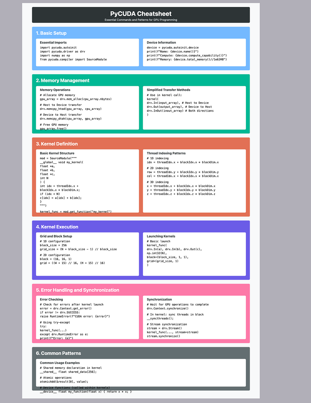
Conclusion
The exploration of CUDA programming through PyCUDA demonstrates the powerful capabilities of GPU parallel processing for computational tasks. Through our practical examples, we’ve seen how GPU acceleration can significantly improve performance for various operations:
- Basic Vector Operations: Simple vector addition and element-wise operations showed the fundamental concepts of GPU parallelization.
2. Matrix Operations: More complex operations like matrix multiplication and convolutions demonstrated the real-world applications in deep learning.
The key takeaways from our exploration include:
- GPU acceleration becomes most effective with large-scale computations where parallelization can be fully utilized
- Proper memory management between host and device is crucial for optimal performance
- Thread hierarchy and block organization are fundamental concepts for efficient CUDA programming
- Hardware-specific limitations must be considered when designing CUDA kernels
While PyCUDA provides a Python interface to CUDA programming, understanding the underlying concepts helps developers optimize their code and make better use of GPU resources in machine learning applications.
References
Official Documentation
1. NVIDIA CUDA Documentation
https://docs.nvidia.com/cuda/
2. PyCUDA Documentation
https://documen.tician.de/pycuda/
Technical Specifications
1. CUDA C++ Programming Guide
https://docs.nvidia.com/cuda/cuda-c-programming-guide/
2. NVIDIA GPU Architecture
https://www.nvidia.com/en-us/technologies/cuda-x/
Additional Resources
1. “Parallel Programming and Computing Platform | CUDA”
NVIDIA Developer Documentation
2. “Optimizing CUDA Applications”
NVIDIA Developer Blog
3. “GPU Computing with Python”
PyCUDA Tutorial Documentation
4. “CUDA by Example: An Introduction to General-Purpose GPU Programming”
Sanders, J., & Kandrot, E. (2010)
PyCUDA Glossary
Basic Terms
- PyCUDA: A Python wrapper for NVIDIA’s CUDA API, allowing Python programs to use GPU computing
- Host: The CPU and its memory (main computer memory)
- Device: The GPU and its memory (graphics card memory)
- Kernel: A function that runs on the GPU, marked with __global__ in CUDA code
- Thread: The smallest unit of parallel execution on GPU
Memory-Related Terms
- cudaMalloc: Function to allocate memory on the GPU
- cudaFree: Function to free allocated GPU memory
- cudaMemcpy: Function to copy data between CPU and GPU memory
- drv.In: PyCUDA method to mark input arrays being sent to GPU
- drv.Out: PyCUDA method to mark output arrays being received from GPU
- drv.InOut: PyCUDA method for arrays that serve as both input and output
Thread Organization
- Block: A group of threads that execute the same kernel
- Grid: A collection of blocks
- threadIdx: Index of the current thread within its block
- blockIdx: Index of the current block within the grid
- blockDim: Dimensions (size) of a block
- gridDim: Dimensions (size) of the grid
PyCUDA-Specific Components
- SourceModule: PyCUDA class used to compile CUDA C code
- autoinit: PyCUDA module that automatically initializes CUDA context
- driver: PyCUDA module providing low-level CUDA driver API access
- get_function: Method to get a callable kernel function from compiled CUDA code
Synchronization and Control
- cudaDeviceSynchronize: Function to ensure all GPU operations are completed
- __syncthreads: Function to synchronize all threads within a block
- cudaGetLastError: Function to check for CUDA errors
Memory Types
- Global Memory: Main GPU memory accessible by all threads
- Shared Memory: Fast memory shared between threads in the same block
- Local Memory: Private memory for each thread
- Constant Memory: Read-only memory accessible by all threads
Performance Terms
- Warp: Group of 32 threads that execute together (basic unit of thread scheduling)
- Occupancy: Ratio of active warps to maximum possible warps
- Memory Coalescing: Pattern of memory access where consecutive threads access consecutive memory locations
- Bank Conflicts: When multiple threads in a warp access the same memory bank
Common CUDA Function Qualifiers
- global: Marks a function that runs on GPU, callable from CPU
- device: Marks a function that runs on GPU, callable only from GPU
- host: Marks a function that runs on CPU (default)
- shared: Declares a variable in shared memory
Error Handling
- cudaError_t: CUDA error type for error checking
- cudaSuccess: Status indicating successful CUDA operation
- cudaGetErrorString: Function to get human-readable error message
PyCUDA from Ground Up: A Comprehensive Guide was originally published in Level Up Coding on Medium, where people are continuing the conversation by highlighting and responding to this story.
This content originally appeared on Level Up Coding - Medium and was authored by Senthil E
Senthil E | Sciencx (2024-10-28T00:59:34+00:00) PyCUDA from Ground Up: A Comprehensive Guide. Retrieved from https://www.scien.cx/2024/10/28/pycuda-from-ground-up-a-comprehensive-guide/
Please log in to upload a file.
There are no updates yet.
Click the Upload button above to add an update.
